Parametric SurPyval Modelling
The parametric API is essentially the exact same as the non-parametric API. All models are fit by a
call to the fit() method. However, the parametric models have more options that are only applicable to parametric modelling. The inputs of x for the random variable, c for the censoring flag, n
for count of each x, xl and xr for intervally censored data (can’t be used with x) t
for the truncation matrix, tl for the left truncation scalar or array, and tr for the right truncation scalar or array all remain.
These ingredients compose freely — any mix of censoring, counts and truncation
in a single fit call — and the same convention is used by every model in
the package (non-parametric, regression, recurrent, competing-risks and
copula). See Data Wrangling Examples for worked examples that combine
them and convert between input formats.
On top of the data, fit takes the options that describe the model and
how to estimate it. Each is demonstrated below:
how: the estimation method, one of'MLE'(the default),'MPS','MSE','MPP'or'MOM';offset=True: add a threshold (shift) parametergamma;lfp=True: a limited failure population, where only a proportionpcan ever fail;zi=True: zero inflation, where a proportionf0fails at time zero;fixed: a dictionary of parameters to hold at known values;init: a starting point for the optimiser;heuristic,rr,on_d_is_0andturnbull_estimator: options for probability plotting.
What each estimation method optimises, and why each accepts the data it does, is explained in Parametric Estimation. The API reference for every distribution is listed in Parametric, and the fitted model object is documented in Parametric model API.
Available distributions
Every distribution is an object in the surpyval namespace
(surv.Weibull, surv.Gamma, …) with the same fit,
from_params and distribution functions. The continuous ones are:
Distribution |
Parameters ( |
Support |
|
|
Solved in closed form |
|---|---|---|---|---|---|
|
|
\((0, \infty)\) |
yes / yes |
yes |
MLE (exact and right-censored data, left truncation) |
|
|
\((0, \infty)\) |
yes / yes |
yes |
|
|
|
\((0, \infty)\) |
yes / yes |
no |
|
|
|
\((0, \infty)\) |
yes / yes |
no |
|
|
|
\((0, \infty)\) |
yes / yes |
yes |
MLE (complete data); MOM |
|
|
\((0, \infty)\) |
yes / yes |
yes |
|
|
|
\((0, \infty)\) |
yes / yes |
yes |
|
|
|
\((-\infty, \infty)\) |
no / no |
yes |
MLE (complete data) |
|
|
\((-\infty, \infty)\) |
no / no |
yes |
|
|
|
\((-\infty, \infty)\) |
no / no |
yes |
|
|
|
\((-\infty, \infty)\) |
no / no |
yes |
|
|
|
\([a, b]\) |
no / no |
yes |
MLE; MOM |
|
|
\([0, 1]\) |
no / yes |
no |
MOM |
|
|
\([a, b]\) |
no / no |
no |
|
|
|
\((0, \infty)\) |
built with |
||
|
your own |
your own |
if the support is \((0, \infty)\) |
no |
Galton and Gauss are the same distributions as LogNormal and
Normal under their other names. Every distribution in the table except the
Hypoexponential also accepts lfp=True. The discrete lifetimes
(Geometric, DiscreteWeibull, NegativeBinomial, BetaGeometric,
Discretize and Poisson) and the per-demand and degenerate models
(Bernoulli, FixedEventProbability, Binomial, ExactEventTime,
InstantlyOccurs and NeverOccurs) have their own sections below, and the
flexible Royston-Parmar model and mixtures of any of these have theirs.
Complete Data
The easiest and simplest case is that when you have a dataset of exactly observed data. that is,
you have one array of data with the values at which they failed. Fitting a parametric distribution
to the data can be done with a simple call to the fit() method:
import surpyval as surv
import numpy as np

np.random.seed(10)
x = surv.Weibull.random(50, 30., 9.)
model = surv.Weibull.fit(x)
model
Parametric SurPyval Model
=========================
Distribution        : Weibull
Fitted by           : MLE
Data                : 50 units: 50 events at 50 unique times
Parameters          :
     alpha: 29.8051373999103
      beta: 10.29603800569635
To visualise the outcome of this fit we can inspect the results on a probability plot:
model.plot()
<Axes: title={'center': 'Weibull Probability Plot'}, xlabel='Time', ylabel='CDF'>
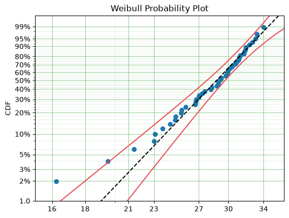
The points, the fitted line and its confidence bounds are drawn in one colour,
the next of the axes’ colour cycle, so several models can share one plot;
label= names the fitted line in a legend, color= sets the colour, and
other keyword arguments (linestyle, linewidth, …) go to the fitted
line. To compare two populations:
from matplotlib import pyplot as plt

other = surv.Weibull.fit(surv.Weibull.random(50, 40., 5.))
fig, ax = plt.subplots()
model.plot(ax=ax, label="first")
other.plot(ax=ax, label="second")
ax.legend();

The model object from the above example can be used to calculate the density of the distribution with the parameters found with the best fit from above. This is very easy to do:
from matplotlib import pyplot as plt

x_plot = np.linspace(10, 50, 1000)
f = model.df(x_plot)
plt.plot(x_plot, f)
[<matplotlib.lines.Line2D at 0x7b2ace75af30>]

The CDF ff(), Survival (or Reliability) sf(), hazard
rate hf(), or cumulative hazard rate Hf() can be computed as
well. This functionality makes it very easy to work with surpyval models to
determine risks or to pass the function to other libraries to find optimal
trade-offs.
Working with a fitted model
The fitted parameters are in model.params, in the order given by
model.parameter_names (the distribution’s parameter_names), and each
is also available by name:
print(model.parameter_names, model.params)
print("alpha =", model.alpha, " beta =", model.beta)
['alpha', 'beta'] [29.8051374  10.29603801]
alpha = 29.8051373999103  beta = 10.29603800569635
Every function of the distribution is a method of the model. As well as the
five functions above there is the quantile function qf (the inverse of
the CDF, so model.qf(0.1) is the “B10 life” by which 10% have failed), the
conditional survival cs(x, given) (the probability of surviving a
further x given survival to given, the ratio
\(R(given + x)/R(given)\) of the model’s own survival function, so it
counts any never-failing or zero-inflated proportion and any offset), and
the summary statistics:
t = np.array([20., 30., 40.])
print("R(t)   :", model.sf(t))
print("F(t)   :", model.ff(t))
print("h(t)   :", model.hf(t))
print("H(t)   :", model.Hf(t))
print("B10    :", model.qf(0.1))
print("median :", model.qf(0.5))
print("P(survive 5 more | survived 25):", model.cs(5, given=25))
print("mean, variance :", model.mean(), model.var())
print("E[X^2], entropy:", model.moment(2), model.entropy())
R(t)   : [9.83687137e-01 3.43215305e-01 1.04607986e-09]
F(t)   : [0.01631286 0.65678469 1.        ]
h(t)   : [0.00846714 0.36701851 5.32259248]
H(t)   : [1.64473826e-02 1.06939732e+00 2.06782161e+01]
B10    : 23.953499645948316
median : 28.762812007330044
P(survive 5 more | survived 25): 0.404235101975587
mean, variance : 28.38987795504249 11.040563172950897
E[X^2], entropy: 817.0257334751584 2.584075357356664
The model also records how it was made: the estimation method, the optimiser
that converged (see Parametric Estimation), whether a maximum
likelihood fit reached a verified maximum (maximum: 'verified',
'unverified' or 'no finite maximum', the last two with a warning; see
Parametric), the support,
and, for a maximum likelihood fit, the parameter covariance hess_inv whose
diagonal holds the squared standard errors:
print("fitted by :", model.method, "using", model.optimizer)
print("maximum   :", model.maximum)
print("support   :", model.support)
print("std errors:", np.sqrt(np.diag(model.hess_inv)))
fitted by : MLE using BFGS
maximum   : verified
support   : [ 0. inf]
std errors: [0.4286872  1.18990405]
The distributions can also be used directly, without a model, by passing
the parameters after x. This is handy for a quick calculation:
surv.Weibull.sf(t, 30., 9.)
array([9.74323110e-01, 3.67879441e-01, 1.64413693e-06])
Models from known parameters
Not every model comes from data. A supplier’s datasheet, a handbook value or
an earlier analysis may give you the parameters, and from_params builds a
full model from them, with all of the methods above. It also takes the
structural options as values: gamma for an offset, p for a limited
failure population and f0 for zero inflation (each explained below).
known = surv.Weibull.from_params([30., 9.])
print("R(25) =", known.sf(25.))

shifted = surv.Weibull.from_params([10., 2.], gamma=5.)
print(shifted)
print("R at 4, 5 and 10:", shifted.sf([4., 5., 10.]))
R(25) = 0.8238171331688301
Parametric SurPyval Model
=========================
Distribution        : Weibull
Fitted by           : given parameters
Offset (gamma)      : 5.0
Parameters          :
     alpha: 10.0
      beta: 2.0
R at 4, 5 and 10: [1.         1.         0.77880078]
Nothing can fail before the offset, so the survival of the shifted model is
exactly one up to gamma = 5.
Some distributions exist only in this form. The Hypoexponential is the
lifetime of something that must pass through several independent,
memoryless stages in turn: a load-sharing group whose failure rate changes as
members fail, or a warm-standby system. Each stage lasts an exponential time
with its own rate, and the lifetime is their sum. Because the number of
stages is up to you, it takes any number of rates, and there is no fit:
you construct it from rates you know (see Hypoexponential Distribution).
from surpyval import Hypoexponential

# Three stages with rates 0.5, 1.5 and 3.0 per unit time
standby = Hypoexponential.from_params([0.5, 1.5, 3.0])
print(standby)
print("mean:", standby.mean())
print("R at 1, 2 and 5:", standby.sf([1., 2., 5.]))
Parametric SurPyval Model
=========================
Distribution        : Hypoexponential
Fitted by           : given parameters
Parameters          :
  lambda_1: 0.5
  lambda_2: 1.5
  lambda_3: 3.0
mean: 3.0
R at 1, 2 and 5: [0.87858244 0.61289168 0.14719997]
The mean is the sum of the stage means, \(1/0.5 + 1/1.5 + 1/3 = 3\), as
it should be. The rates must be distinct: as two rates approach each other the
closed form becomes numerically unstable, and SurPyval raises an error. When
every stage has the same rate the sum is an Erlang distribution, which is a
Gamma with an integer shape:
erlang = surv.Gamma.from_params([3, 1.0])   # three stages, each with rate 1
print("R at 1, 2 and 5:", erlang.sf([1., 2., 5.]))
R at 1, 2 and 5: [0.9196986 0.67667642 0.12465202]
Random samples
Random samples are drawn with random, either from a distribution with
given parameters or from a model. They are useful for simulation studies,
for testing an analysis on data where you know the answer (as the examples
on this page do), and for Monte Carlo propagation of risk. Seed numpy’s
generator to make them repeatable. A model can also be sampled truncated,
between a and b:
np.random.seed(1)
print(surv.Weibull.random(5, 30., 9.))   # from the distribution
print(model.random(5))                   # from a fitted model
print(model.random(5, a=25, b=30))       # only values between 25 and 30
[28.01250792 30.81849956 10.94361301 26.78078126 24.45115542]
[23.75915927 25.56666774 27.42185277 27.89402354 29.07253693]
[27.58677095 28.74311497 26.45979148 29.51502169 25.2336869 ]
A model with a limited failure population returns its sample as
(x, c, n, t) arrays instead of a single array, because some of the drawn
units never fail and have to be recorded as right censored. The limited
failure population section below uses this.
Saving and loading a model
A fitted model can be stored and restored with to_dict and
surpyval.from_dict, or written to a JSON file with to_json and read
back with surpyval.from_json. The package-level readers work out which
kind of model wrote the file, so the same call restores a Weibull, a mixture,
a Royston-Parmar model or any other SurPyval model (see
Saving and Loading Models).
import os
import tempfile

restored = surv.from_dict(model.to_dict())
print(restored.sf(25.), model.sf(25.))

path = os.path.join(tempfile.mkdtemp(), "weibull.json")
model.to_json(path)
print(surv.from_json(path).params)
0.8490487436208652 0.8490487436208652
[29.8051374  10.29603801]
The dictionary holds the parameters, their covariance, the fitted
negative log-likelihood and the sample size of the information criteria but,
by default, not the data. So a restored model can still give Wald confidence
bounds and every information criterion (neg_ll(), aic(), aic_c(),
bic()), but not plot() or likelihood-ratio bounds – each says so if
asked. Pass with_data=True to to_dict (or to_json) to keep the
data, which restores plot() and the likelihood-ratio bounds. A model of a Discretize
distribution is saved and restored the same way; one of a
CustomDistribution is restored once the same distribution has been
constructed again (see CustomDistribution).
Using censored data
Right Censored
A common complication in survival analysis is that all the data is not observed up to the point of failure (or death). In this case the data is right censored, see the Types of Data section for a more detailed discussion, surpyval offers a very clean and easy way to model this. First, let’s create a simulated data set:
import surpyval as surv
import numpy as np

np.random.seed(10)
x = surv.Weibull.random(50, 30, 2.)
observation_limit = 40
# Censoring flag
c = (x >= observation_limit).astype(int)
x[x >= observation_limit] = observation_limit
In this example, we created 50 random Weibull distributed values with alpha = 30 and beta = 2. For this example the observation window has been set to 40. This value is where we stopped observing the events. For all the randomly generated values that are above this limit we create the censoring flag array c. This array has zeros where the event time was observed, and a 1 where the value is above the recorded value. For all the values in the data that are above 40 we set them to 40. This is a common occurrence in survival analysis and surpyval is designed to accept this input with a simple call:
model = surv.Weibull.fit(x, c)
model
Parametric SurPyval Model
=========================
Distribution        : Weibull
Fitted by           : MLE
Data                : 50 units: 45 events at 45 unique times, 5 right censored
Parameters          :
     alpha: 29.249248400841505
      beta: 2.2291489730398717
The plot for this can be seen to be:
model.plot(show_censored=True)
<Axes: title={'center': 'Weibull Probability Plot'}, xlabel='Time', ylabel='CDF'>

The points are the failures only. A suspension (a right-censored unit)
moves the plotting positions of the failures after it, but has no position
of its own, so it is not drawn as a point (the convention of Abernethy’s
New Weibull Handbook and of Weibull++); show_censored=True marks the
suspension times with ticks along the time axis, here the censored units at
40. The time axis still spans every time.
For a plot of your own, get_plot_data() returns every row of the
plotting positions as x_ and F, suspensions included, with a boolean
mask failed selecting the failures (the points drawn above,
d["x_"][d["failed"]] and d["F"][d["failed"]]) and the suspension
times as x_censored:
d = model.get_plot_data()
print(len(d["x_"]), "rows,", d["failed"].sum(), "failures")
print("suspension times:", d["x_censored"])
46 rows, 45 failures
suspension times: [40.]
The results from this model are very close to the data we input, and with only 50 samples.
Left Censored
The above example can be extended to another kind of censoring; left censored data. This is the case where the values are known to fall below a particular value. We can change our example data set to have a start observation time for which we will left censor all the data below that:
observation_start = 10
# Censoring flag
c[x <= observation_start] = -1
x[x <= observation_start] = observation_start
That is, we set the start of the observations at 10 and flag that all the values at or below this are left censored. We can then use the updated values of x and c:
model = surv.Weibull.fit(x, c)
model
Parametric SurPyval Model
=========================
Distribution        : Weibull
Fitted by           : MLE
Data                : 50 units: 40 events at 40 unique times, 5 right censored, 5 left censored
Parameters          :
     alpha: 29.347097632391574
      beta: 2.3049027885747306
model.plot(heuristic="Turnbull")
<Axes: title={'center': 'Weibull Probability Plot'}, xlabel='Time', ylabel='CDF'>

The values did not substantially change, although the plot does look different as there are no values below 10. Note the heuristic="Turnbull": left-censored units have no rank, so the plotting positions have to come from the Turnbull estimator.
Intervally Censored
The next type of censoring that is naturally handled by surpyval is interval censoring. Creating another example data set:
import surpyval as surv
import numpy as np

np.random.seed(30)
x = surv.Weibull.random(100, 30, 10.)
n, xx = np.histogram(x, bins=[20, 23, 26, 29, 32, 35, 38])
x = np.vstack([xx[0:-1], xx[1:]]).T
In this example we have created the variable x with a matrix of the intervals within which each of the observations have failed. That is each exact observation has been binned into a window and the x array has an entry [left, right] within which the event failed. We also have the n array that has the count of the failures within the window. With these two values we can make the simple surpyval call:
model = surv.Weibull.fit(x, n=n)
model
Parametric SurPyval Model
=========================
Distribution        : Weibull
Fitted by           : MLE
Data                : 100 units: 0 events, 100 interval censored
Parameters          :
     alpha: 29.959291590923154
      beta: 9.498149821579963
model.plot(heuristic="Turnbull")
<Axes: title={'center': 'Weibull Probability Plot'}, xlabel='Time', ylabel='CDF'>

Again, we have a result that is very close to the original parameters. SurPyval can take as input an arbitrary combination of censored data. This plot also looks to be a great fit! The data at the tails are a little bit off, but the data are binned into only six intervals and the core of the model matches the data quite well.
The same intervals can be given as two separate arrays, xl for the left
ends and xr for the right ends, which is often how inspection data arrive.
It is the same data, so it is the same fit:
surv.Weibull.fit(xl=xx[:-1], xr=xx[1:], n=n).params
array([29.95929159, 9.49814982])
A row with xl == xr is treated as an exact observation, a row with
xr = np.inf as right censored and a row with xl = -np.inf as left
censored, so these two arrays can describe any mix of censoring.
Mixed Censoring
Mixed censoring, or arbitrary censoring is easily handled by SurPyval. So no matter the combination of the data that you have, SurPyval will be able to fit a distribution to it.
import surpyval as surv

x  = [0, 1, 2, [3, 4], [6, 10], [4, 8], 5, 19, 10, 13, 15]
c  = [0, 0, 1, 2, 2, 2, 0, -1, 0, 1, 0]
surv.Gumbel.fit(x, c=c)
Parametric SurPyval Model
=========================
Distribution        : Gumbel
Fitted by           : MLE
Data                : 11 units: 5 events at 5 unique times, 2 right censored, 1 left censored, 3 interval censored
Parameters          :
        mu: 9.912232243410875
     sigma: 4.959520118151789
Using truncated data
Left truncated
Surpyval has the capacity to handle arbitrary truncated data. A common occurrence of this is in the insurance industry data. When customers make a claim on their policies they have to pay an ‘excess’ which is a charge to submit a claim for processing. If say, the excess on a set of policies in an area is $250, then it would not be logical for a customer to submit a claim for a loss of less than that number. Therefore there will be no claims under $250. This can also happen in engineering where a part may be tested up to some limit prior to be sold, therefore, as a customer you need to make sure you take into account the fact that some parts would have been rejected at the end of the line which you may not have seen. So a washing machine may run through 25 cycles prior to shipping. This is similar to, but distinct from censoring. When something is left censored, we know there was a failure or event below the threshold. Whereas with truncation, we do not see any variables below the threshold. A simulated example may explain this better:
import numpy as np
import surpyval as surv

np.random.seed(10)
x = surv.Weibull.random(100, 100, 0.6)
# Keep only those values greater than 25
threshold = 25
x = x[x > threshold]
We have therefore simulated a scenario where we have taken 100 random samples from a fat tailed Weibull distribution. We then filter to keep only those records that are above the threshold. In this case we assume we haven’t seen the data for the washing machines with less than 25 cycles. To understand what could go wrong if we ignore this, what do we get if we assume all the data are failures and there is no truncation?
model = surv.Weibull.fit(x=x)
print(model.params)
[198.49516984 1.01696672]
With a plot that looks like:
model.plot()
<Axes: title={'center': 'Weibull Probability Plot'}, xlabel='Time', ylabel='CDF'>

Looking at the parameters of the distribution, you can see that the beta value is greater than 1. Although only slightly, this implies that this distribution has an increasing hazard rate. If you were the operator of the washing machines (e.g. a hotel or a laundromat) and any downtime had a cost, you would conclude from this that replacing the machines after a fixed time would be a good policy.
But if you take the truncation into account:
model = surv.Weibull.fit(x=x, tl=threshold)
print(model.params)
[94.898437 0.64100022]
With the plot:
model.plot(heuristic="Turnbull")
<Axes: title={'center': 'Weibull Probability Plot'}, xlabel='Time', ylabel='CDF'>
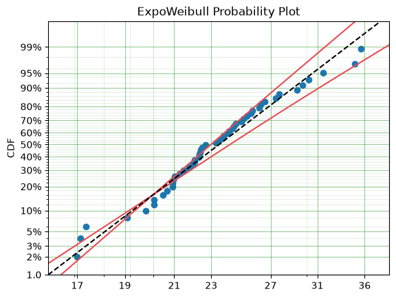
You can see now that the model fits the data much better, but also that the beta parameter is actually below 1. This shows that ignoring the left-truncated data in parametric estimation can lead to errors in prediction.
Right truncated
The example from above can be continued for right-truncated data as well. Here the data come from a Normal distribution with a mean of 100 and a standard deviation of 10, but only values between 85 and 115 could be recorded:
import numpy as np
import surpyval as surv

np.random.seed(10)
x = surv.Normal.random(100, 100, 10)
tl = 85
tr = 115
# Truncate the data
x = x[(x > tl) & (x < tr)]
print(len(x), "values were recorded")

naive = surv.Normal.fit(x)
model = surv.Normal.fit(x=x, tl=tl, tr=tr)
print("ignoring the truncation :", naive.params)
print("with the truncation     :", model.params)
87 values were recorded
ignoring the truncation : [99.98933119  6.88071694]
with the truncation     : [99.98495212  8.17170127]
When plotted we get:
model.plot(heuristic="Turnbull")
<Axes: title={'center': 'Normal Probability Plot'}, xlabel='Time', ylabel='CDF'>

From the output above, the number of data points we have has been reduced from the simulated 100, down to 87. Both fits find the centre, but the naive fit badly underestimates the spread: the truncation removed the tails, so the recorded values look less variable than the population really is. Accounting for the truncation moves the estimate of \(\sigma\) back towards the true value of 10. It cannot recover it completely – the tails that carry most of the information about the spread were never recorded – which is a useful reminder that truncation costs information even when it is modelled correctly.
In the cases above we used a scalar value for the truncation values. But some data has individual values for left truncation. This is seen in trials where someone may join the trial as a late entry. Therefore each data point as an entry time. For example:
import surpyval as surv

x  = [3, 4, 6, 7, 9, 10]
tl = [0, 0, 0, 0, 5, 2]

model = surv.Weibull.fit(x, tl=tl)
print(model.params)
[7.05854701 2.70096668]
Intervally and Arbitrarily truncated
Surpyval can even work with arbitrary left and right truncation:
import surpyval as surv

x  = [3, 4, 6, 7, 9, 10]
tl = [0, 0, 0, 0, 5, 2]
tr = [10, 9, 8, 10, 15, 15]

model = surv.Weibull.fit(x, tl=tl, tr=tr)
print(model.params)
[8.12377637 2.56917058]
In the above example we used both the tl and tr. However, surpyval has a flexible API where it can take the truncation data as a two dimensional array:
import surpyval as surv

x  = [3, 4, 6, 7, 9, 10]
t =  [[0, 10], [0, 9], [0, 8], [0, 10], [5, 15], [2, 15]]

model = surv.Weibull.fit(x, t=t)
print(model.params)
[8.12377637 2.56917058]
Which, obviously, gives the same result. This shows the flexibility of the surpyval API, you can use scalar, array, or matrix values for the truncations using the t, tl, and tr keywords with the fit method and surpyval does the rest.
Truncation needs a method that models it. Maximum likelihood handles any
truncation; MPS handles a single window shared by every observation (scalar
tl and tr); probability plotting handles it only through the
non-parametric estimate, with the limitation shown at the end of the section
on alternate estimation methods below; and MSE and MOM do not accept
truncated data at all.
Offsets
Another common feature in survival analysis is a requirement to fit a distribution with an offset. These distributions are sometimes referred to as the two-parameter (e.g. two parameter exponential) three parameter, (e.g., the three parameter Weibull), or four parameter (e.g four parameter Exponentiated Weibull distribution). SurPyval however just uses an offset to increase the numbers of parameters and allow the distribution to be shifted.
Using data from Weibull’s original paper for the strength of Bofors steel shows when this might be necessary.
import surpyval as surv
from surpyval.datasets import load_bofors_steel

df = load_bofors_steel()
x = df['x']
n = df['n']

model = surv.Weibull.fit(x=x, n=n)
print(model.params)
[47.36735846 17.57131953]
model.plot()
<Axes: title={'center': 'Weibull Probability Plot'}, xlabel='Time', ylabel='CDF'>

The above plot does not look to be a good fit. However, if we use an offset we can use the three parameter Weibull distribution to attempt to get a better fit. Using offset values with surpyval is very easy:
import surpyval as surv
from surpyval.datasets import load_bofors_steel

df = load_bofors_steel()
x = df['x']
n = df['n']

model = surv.Weibull.fit(x=x, n=n, offset=True)
print(model)
Parametric SurPyval Model
=========================
Distribution        : Weibull
Fitted by           : MLE
Data                : 389 units: 389 events at 10 unique times
Offset (gamma)      : 39.76563186360473
Parameters          :
     alpha: 7.141922613743938
      beta: 2.6204509637235365
model.plot()
<Axes: title={'center': 'Weibull Probability Plot'}, xlabel='Time', ylabel='CDF'>
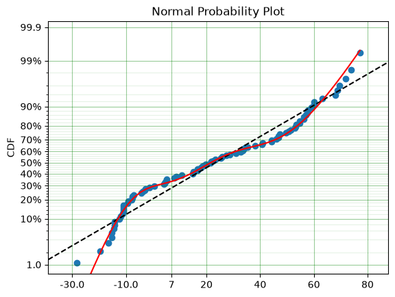
This is evidently a much better fit! The offset value for an offset distribution is saved as gamma in the model object, and every method of the model – sf, qf, mean and the rest – includes the shift. Offsets can be used for any continuous distribution whose support is the half real line \((0, \infty)\): the Weibull, Gamma, LogNormal, LogLogistic, Exponential, Rayleigh and exponentiated Weibull, and a custom distribution declared on that support. For example:
import surpyval as surv
import numpy as np

np.random.seed(10)
x = surv.LogLogistic.random(100, 10, 3) + 10
model = surv.LogLogistic.fit(x, offset=True, how='MLE')
print(model)
Parametric SurPyval Model
=========================
Distribution        : LogLogistic
Fitted by           : MLE
Data                : 100 units: 100 events at 100 unique times
Offset (gamma)      : 9.562706282424404
Parameters          :
     alpha: 10.189471516582426
      beta: 3.4073271438363504
model.plot()
<Axes: title={'center': 'LogLogistic Probability Plot'}, xlabel='Time', ylabel='CDF'>
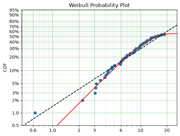
A four parameter exponentiated Weibull can also be found:
import surpyval as surv
import numpy as np

np.random.seed(10)
x = surv.ExpoWeibull.random(100, 10, 1.2, 4) + 10
model = surv.ExpoWeibull.fit(x, offset=True)
print(model)
Parametric SurPyval Model
=========================
Distribution        : ExpoWeibull
Fitted by           : MLE
Data                : 100 units: 100 events at 100 unique times
Offset (gamma)      : 10.701284193362163
Parameters          :
     alpha: 11.475125717235626
      beta: 1.3969799318684342
        mu: 2.8452990012694324
model.plot()
<Axes: title={'center': 'ExpoWeibull Probability Plot'}, xlabel='Time', ylabel='CDF'>

Offsets only make sense for distributions supported on the half real line [0, inf) - the offset gamma simply slides the lower bound of the support. A distribution on the whole real line, such as the Normal, can already sit anywhere, so surv.Normal.fit(x, offset=True) raises a ValueError. A distribution with a finite upper bound, such as the Beta distribution on [0, 1], cannot be offset either, and surv.Beta.fit(x, offset=True) will also raise a ValueError. Sliding the lower bound while pinning the upper bound at 1 does not produce another member of the Beta family. If your data are bounded on both sides and you need to estimate where those bounds are, use the four parameter Beta distribution (Beta4) instead, which estimates the lower bound a and upper bound b along with the two shape parameters:
import surpyval as surv
import numpy as np

np.random.seed(10)
x = surv.Beta4.random(10000, 3., 4., 10., 20.)
model = surv.Beta4.fit(x)
print(model)
Parametric SurPyval Model
=========================
Distribution        : Beta4
Fitted by           : MLE
Data                : 10000 units: 10000 events at 10000 unique times
Parameters          :
     alpha: 2.8883504573151426
      beta: 4.018232451349274
         a: 10.03630152230403
         b: 20.069229923437554
With both shapes above 1, as here, maximum likelihood is fine. The
Beta4’s likelihood is unbounded when a shape is below 1, though: the
density is infinite at that end of the support, so the fit can run the end
onto the smallest or largest observation and stop wherever its search
gave up. Such a fit warns “No finite maximum”, and records it in
model.maximum. Fit with how="MPS"
instead: maximum product of spacings has no such limit, and its estimates
are the same whatever the units of the data.
A caution: offset parameters can be unidentifiable
The offset gamma is a threshold parameter, and threshold parameters are statistically awkward. gamma trades off against the shape and scale parameters, so two very different parameter tuples can describe almost the same distribution. A high-shape Gamma sitting near the origin is, by the central limit theorem, nearly the same bell-shaped curve as a moderate Gamma shifted out to 10. The likelihood surface is correspondingly flat along that trade-off, which makes a threshold fit far more sensitive to its starting point than an ordinary two-parameter fit.
In practice that sensitivity is the estimator’s problem to solve, not yours. Shifted Gamma data is recovered by every fit method that the Gamma supports:
import surpyval as surv
import numpy as np

np.random.seed(0)
x = surv.Gamma.random(10_000, 3.0, 2.0) + 10.0

print('Truth : gamma=10.000, alpha=3.000, beta=2.000')
offset_fits = {}
for how in ['MOM', 'MSE', 'MPS', 'MLE']:
    m = offset_fits[how] = surv.Gamma.fit(x, offset=True, how=how)
    print('{:6s}: gamma={:.3f}, alpha={:.3f}, beta={:.3f}'.format(
        how, m.gamma, *m.params))
Truth : gamma=10.000, alpha=3.000, beta=2.000
MOM   : gamma=10.039, alpha=2.804, beta=1.931
MSE : gamma=9.994, alpha=2.981, beta=1.992
MPS   : gamma=9.986, alpha=3.013, beta=2.003
MLE   : gamma=9.990, alpha=2.996, beta=1.997
MPP is absent from that list because the Gamma does not offer it. A
probability plot needs a straight-line y-axis that can be drawn before
the parameters are known; the Gamma’s CDF is the regularised incomplete
gamma function, with the shape inside the special function rather than
outside as an exponent, so the only such axis is the inverse incomplete
gamma — which needs the shape. To draw the axis you need the answer.
Gamma.fit(x, how="MPP") raises rather than guessing a shape to draw
the axis with; Gamma.plot() is unaffected, since by then the fitted
parameters are in hand.
What makes this work is the starting point. Every optimised offset fit (all but MPP, which needs no start) begins with gamma just below the data, by the data’s mean spacing (their range over \(n - 1\)), and the initialisers read the remaining parameters off x - gamma. Moments taken from the unshifted data would be dominated by the offset, and a shape read from them explodes (the method-of-moments shape, the squared mean over the variance, is about 176 on the sample above, for a true shape of 3); from such a start the optimiser can stop on an absurd tuple that is nonetheless an acceptable distribution, precisely because of the flat trade-off described above.
The underlying caution still stands, though, and it is worth keeping in mind for your own data:
Judge an offset fit by what it predicts, not only by the printed parameters. Plot it against the non-parametric estimate, or compare the survival function, quantiles, mean and variance. Two parameter tuples that look very different can imply nearly the same distribution.
If you need ``gamma`` itself to be meaningful - you are interpreting it as a guaranteed minimum life, say - prefer
MLE, which remains the most accurate on the parameters, and treat a single point estimate of a threshold with care regardless of method. Note thatgammahas no standard error, soparam_cbcannot give an interval for it (see Parametric Estimation).If the MLE struggles - a small sample, or a shape that puts an infinite density at the threshold - try
how='MPS', which was designed for exactly this case (see the section on alternate estimation methods below). The likelihood of an offset fit has no finite maximum whengammacan run onto the first failure: with a Weibull, Gamma or LogLogistic shape below 1 the density there is infinite (for the LogNormal, the scale grows without bound on the way). Such a fit warns “No finite maximum”, returns where its search stopped, withgammaon the smallest observation, and recommendshow='MPS', whose spacings have no such limit. On the seven failures[55, 60, 70, 80, 95, 120, 140]the three-parameter Weibull does this (its shape falls to 0.09), while its MPS fit putsgammaat 49.8, with a shape of 0.95. The two-parameter Exponential is the exception: its density is finite at the threshold, so its maximum atgammaequal to the first failure is a genuine one.
test_offset_divergence.py in the test suite pins this down for offset Gamma and Rayleigh fits with measured KL and Wasserstein distances alongside parameter tolerances: MLE is held to 5% on every parameter, and MOM (on the Rayleigh) to 10%, with the implied distributions essentially identical either way.
Fixing parameters
Another useful feature of surpyval is the ability to easily fix parameters. For example:
import surpyval as surv
import numpy as np

np.random.seed(30)
x = surv.Normal.random(50, 10., 2)
model = surv.Normal.fit(x, fixed={'mu' : 10})
print(model)
Parametric SurPyval Model
=========================
Distribution        : Normal
Fitted by           : MLE
Data                : 50 units: 50 events at 50 unique times
Parameters          :
        mu: 10.0
     sigma: 1.9353652679659545
model.plot()
<Axes: title={'center': 'Normal Probability Plot'}, xlabel='Time', ylabel='CDF'>

You can see that the mu parameter has been fixed at 10. This can work for distributions with many more parameters, including the offset.
import surpyval as surv
import numpy as np

np.random.seed(30)
x = surv.ExpoWeibull.random(50, 10., 2, 4) + 10
model = surv.ExpoWeibull.fit(x, offset=True, fixed={'mu' : 4, 'gamma' : 10, 'alpha' : 10})
print(model)
Parametric SurPyval Model
=========================
Distribution        : ExpoWeibull
Fitted by           : MLE
Data                : 50 units: 50 events at 50 unique times
Offset (gamma)      : 10.0
Parameters          :
     alpha: 10.0
      beta: 2.0442048984292556
        mu: 4.0
model.plot()
<Axes: title={'center': 'ExpoWeibull Probability Plot'}, xlabel='Time', ylabel='CDF'>

We have fit only one of the four parameters of an offset exponentiated-Weibull distribution, holding the other three at known values!
Parameters are fixed by name, using the names in the distribution’s
parameter_names plus gamma for the offset. Fixing works with MLE,
MPS, MSE and MOM, but not with probability plotting, which fits
all of the parameters of its line at once. With MOM a fixed parameter
needs no equation of its own, so the method matches one moment per free
parameter (see Parametric Estimation). A fixed parameter is known rather
than estimated, so it has no standard error, the confidence bounds of the other
parameters are conditional on it, and it does not count in the parameter number
\(k\) of aic(), aic_c() and bic().
Fixing a parameter also reduces how much data a fit needs. SurPyval refuses to fit when there are fewer distinct (non-right-censored) values than free parameters, because the answer would be arbitrary; a Weibull cannot be fitted to a single value. With the shape fixed – a common practice in reliability, where a “Weibayes” analysis assumes a shape from experience – one value is enough:
surv.Weibull.fit([10.], fixed={'beta': 2.}).params
array([10., 2.])
With no failure at all there is still no fit, shape fixed or not: every
unit suspended leaves the likelihood rising without bound as the scale grows
past the suspensions, so fit raises. The standard answer to “ten units
ran 500 hours with no failure; assuming a shape of 2, how long is the
characteristic life at least?” is not a maximum-likelihood estimate but a
confidence bound, the Weibayes bound (Nelson, 1985; Abernethy’s New Weibull
Handbook, chapter 6), and surpyval.weibayes computes it:
bound = surv.weibayes([500] * 10, c=[1] * 10, beta=2, alpha_ci=0.05)
print("alpha is at least", bound.params[0].round(1))
print("R(500) is at least", bound.sf(500).round(3))
alpha is at least 913.5
R(500) is at least 0.741
It returns the Weibull at the bound, so its sf is the lower bound on
the reliability (0.741 at 500 hours, the same as success_run(10)) and
its qf the lower bound on a B-life. It takes failures too (the bound
then uses \(2r + 2\) degrees of freedom), and beta=1 gives the
exponential zero-failure bound on the mean life.
Finally, the optimiser can be given a starting point with init: the
values in the order of parameter_names, with gamma first if there is an
offset and p then f0 last for a limited failure population or zero
inflation. With fixed, init may list just the free parameters. You
rarely need it, but if a fit fails, a starting point near the answer – a
shape of 1 and a scale near the mean of the data, say – is the first thing
to try. An explicit init is used as the only start: the extra starting
points SurPyval otherwise tries for limited-failure and custom-distribution
fits (see Parametric Estimation) are skipped.
np.random.seed(30)
x = surv.Weibull.random(50, 30., 2.)
surv.Weibull.fit(x, init=[30., 1.]).params
array([29.38365385, 1.96961618])
Modelling with arbitrary input
The surpyval API is extremely flexible. All the unique examples provided above can all be used at once. That is, data can be censored, truncated, and directly observed with offsets and fixing parameters. The API is completely flexible. This makes surpyval an extremely useful tool for analysts where the data is gathered in a manner where its cleanliness is not guaranteed.
import surpyval as surv
import numpy as np

x  = [0, 1, 2, [3, 4], [6, 10], [4, 8], 5, 19, 10, 13, 15]
c  = [0, 0, 1, 2, 2, 2, 0, -1, 0, 1, 0]
tl = [-1, 0, 0, 0, 0, 0, 2, 2, -np.inf, 0, 0]
tr = 25
model = surv.Normal.fit(x, c=c, tl=tl, tr=tr, fixed={'mu' : 1.})
print(model)
Parametric SurPyval Model
=========================
Distribution        : Normal
Fitted by           : MLE
Data                : 11 units: 5 events at 5 unique times, 2 right censored, 1 left censored, 3 interval censored; 10 left truncated, 11 right truncated
Parameters          :
        mu: 1.0
     sigma: 8.852061293671202
Data often live in a table. fit_from_df takes a pandas DataFrame and
the names of its columns (x_col, c_col, n_col, xl_col /
xr_col, tl_col / tr_col); tl_col and tr_col may be a
column name or a single value, and any other fit option is passed
straight through:
import pandas as pd

df = pd.DataFrame({
    'hours':    [3, 4, 6, 7, 9, 10, 12],
    'censored': [0, 0, 1, 0, 0, 1, 0],
    'entry':    [0, 0, 0, 1, 2, 2, 0],
})
model = surv.Weibull.fit_from_df(
    df, x_col='hours', c_col='censored', tl_col='entry'
)
print(model.params)
[9.25814326 2.32671972]
Sometimes there are no unit-level data at all, only a curve: a failure
curve read off a supplier’s report, say. fit_from_ecdf(x, F) fits the
distribution to the points of such a curve by probability plotting – the
same straight line how='MPP' draws, but through the CDF values you
give (each F must lie in [0, 1], one per x, or it raises a
ValueError). fit_from_non_parametric does the same with a fitted
non-parametric model, through its failure times only, so it matches
how='MPP' with that estimator as the heuristic, on censored data too:
t = np.array([2., 5., 8., 12., 16.])
F = np.array([0.04, 0.22, 0.47, 0.76, 0.92])   # read off a published curve
from_curve = surv.Weibull.fit_from_ecdf(t, F)
print(from_curve.params, "R(10) =", from_curve.sf(10.))

np.random.seed(1)
x = surv.Weibull.random(60, 10., 2.)
c = (x > 15).astype(int)   # right censor at 15
x = np.minimum(x, 15.)
km = surv.KaplanMeier.fit(x, c)
print(surv.Weibull.fit_from_non_parametric(km).params)
print(surv.Weibull.fit(x, c, how='MPP', heuristic='Kaplan-Meier').params)
[10.04534816  1.9847503 ] R(10) = 0.37118300267876503
[9.83533346 1.30848667]
[9.83533346 1.30848667]
A model made this way has all the distribution functions, but it holds no
data, so it has no likelihood, information criteria or confidence bounds.
Only distributions with a probability plot (how='MPP') can be fitted
from a curve.
Using alternate estimation methods
Surpyval’s API is very flexible because you can change which method is used to estimate parameters. This is useful when a more appropriate method is needed or the method you are using fails. The five methods, what they optimise and what data each accepts are explained in Parametric Estimation; here we see them at work.
When MLE is not the best estimator
The default parametric method for surpyval is the maximum likelihood estimation (MLE), this is because it can take any arbitrary input. However, the MLE is not always the best estimator. Consider an example with the uniform distribution:
import surpyval as surv
import numpy as np

np.random.seed(5)
x = surv.Uniform.random(20, 5, 10)
print(x.min(), x.max())

mle_model = surv.Uniform.fit(x)
print(*mle_model.params)
5.403706343824374 9.593054539689607
5.403706343824374 9.593054539689607
You can see that the results are the same. This is because the maximum likelihood estimate of the parameters of a uniform distribution are just the smallest and largest values in the sample. If however we use the ‘Maximum Product Spacing’ method we get:
mps_model = surv.Uniform.fit(x, how='MPS')
print(*mps_model.params)
5.183214333515678 9.813546549998303
You can see that using the MPS method we have parameters that are closer to the real values. This is because the MPS method can ‘look outside’ the existing values to estimate where the real value lies. See the details of this method in the Parametric Estimation section. But the MPS method is useful when you need to estimate the point at which a distribution’s support starts or for any distribution that has unknown support. Concretely, this includes any offset distribution or a distribution with a finite upper and lower support (such as the Uniform).
When an estimation method fails
The other important use case is when, for some reason, an alternate estimation method just does not work. For example, fitting an offset LogLogistic to only ten points:
import surpyval as surv
import numpy as np
import warnings

np.random.seed(30)
x = surv.LogLogistic.random(10, 4., 2) + 10

with warnings.catch_warnings(record=True) as caught:
    warnings.simplefilter("always")
    model = surv.LogLogistic.fit(x, how='MLE', offset=True)
print(str(caught[0].message).splitlines()[0])
model.plot()
MLE Failed; returning the optimiser's starting point (a probability-plot fit, or a rougher initial guess where the distribution has none) instead. Try making the values of the data closer to 1 by dividing or multiplying by some constant.
<Axes: title={'center': 'LogLogistic Probability Plot'}, xlabel='Time', ylabel='CDF'>

This shows, that the Maximum Likelihood Estimation has failed for this data: SurPyval warns and hands back the optimiser’s starting point instead. For many distributions that starting point is a probability-plot fit; for an offset LogLogistic it is only a rough guess, which is why the fitted curve misses the points. The warning is captured and printed above; in your own code it simply appears as a UserWarning. However, because we have access to other methods, we can use an alternate estimation method:
import surpyval as surv
import numpy as np

np.random.seed(30)
x = surv.LogLogistic.random(10, 4., 2) + 10
model = surv.LogLogistic.fit(x, how='MPS', offset=True)
print(model)
Parametric SurPyval Model
=========================
Distribution        : LogLogistic
Fitted by           : MPS
Data                : 10 units: 10 events at 10 unique times
Offset (gamma)      : 11.524905421790487
Parameters          :
     alpha: 2.6318648450075988
      beta: 0.9657652091584717
model.plot()
<Axes: title={'center': 'LogLogistic Probability Plot'}, xlabel='Time', ylabel='CDF'>

Our estimation has worked! The fit converged and follows the ten points. Do not expect it to return the parameters the data were simulated with (an offset of 10, alpha = 4, beta = 2): ten points say little about a three-parameter distribution, and, as the caution on offsets above explains, quite different parameter sets describe nearly the same curve. Even though we used the MPS estimate for the parameters, we can still call all the same functions with the created variable to find the density df(), hazard hf(), CDF ff(), SF sf() etc. So regardless of the estimation method, we can still use the model.
This shows the power of the flexible API that surpyval offers, because if your modelling fails using one estimation method, you can use another. In this case, the MPS method is quite good at handling offset distributions. It is therefore a good approach to use when using offset distributions.
Every method on the same data
Each method has its own options and its own limits. Probability plotting
takes the plotting-position heuristic (any of those listed in
Parametric Estimation, or 'Nelson-Aalen', 'Kaplan-Meier',
'Fleming-Harrington', 'Turnbull' and 'Filliben') and the
regression direction rr. MSE, MPP and MLE accept censored data (MPP
needs heuristic='Turnbull' for left- or interval-censored data); MPS
accepts right- and left-censored but not interval-censored data; MOM needs
exact observations. Here the four that accept censoring fit the same
right-censored sample (the data were simulated with alpha = 10 and
beta = 2), and MOM declines:
np.random.seed(2)
x = surv.Weibull.random(100, 10., 2.)
c = (x > 15).astype(int)
x = np.minimum(x, 15.)

for how in ["MLE", "MPS", "MSE", "MPP"]:
    print(f"{how:<4}", surv.Weibull.fit(x, c, how=how).params)
print("MPP with Blom and rr='x'",
      surv.Weibull.fit(x, c, how="MPP", heuristic="Blom", rr="x").params)

try:
    surv.Weibull.fit(x, c, how="MOM")
except ValueError as e:
    print("MOM :", e)
MLE  [9.14215213 2.17660937]
MPS  [9.16362743 2.10673935]
MSE  [9.00633828 2.30102812]
MPP  [9.1153286  2.11674243]
MPP with Blom and rr='x' [9.09093383 2.20530308]
MOM : Method of moments doesn't support censoring
Asking a method for something it cannot do raises a ValueError (or
NotImplementedError) that says why, rather than returning a quietly wrong
answer.
Likelihoods and information criteria for any method
That extends to the information criteria. A log-likelihood is a property of the
parameters and the data, not of the search that found them, so neg_ll(),
aic(), bic() and aic_c() are available after any fit — not only
after MLE:
np.random.seed(1)
x = surv.Weibull.random(500, 10., 2.)

print(f"{'how':<6}{'neg_ll':>12}{'AIC':>12}{'BIC':>12}")
for how in ["MLE", "MPS", "MSE", "MOM", "MPP"]:
    m = surv.Weibull.fit(x, how=how)
    print(f"{how:<6}{m.neg_ll():12.3f}{m.aic():12.3f}{m.bic():12.3f}")
how         neg_ll         AIC         BIC
MLE       1466.325    2936.651    2945.080
MPS       1466.386    2936.773    2945.202
MSE       1466.676    2937.352    2945.781
MOM       1466.398    2936.796    2945.225
MPP       1470.712    2945.424    2953.853
Two things are worth noticing. The first is that you can compare distributions by AIC or BIC regardless of how you fitted them, which is the usual way of choosing between candidate models. The second is a sanity check on the estimators themselves: MLE attains the lowest negative log-likelihood, because that is precisely the quantity it minimises. The others land close behind, each optimising something else — MPS the spacings, MSE the distance to the non-parametric estimate, MPP the straightness of the probability plot, MOM the moments.
Comparing distributions
To choose a distribution, fit the candidates to the same data and compare an
information criterion; lower is better. fit_best(x, c, n, t) does this by
maximum likelihood for eleven continuous distributions – Beta,
Exponential, ExpoWeibull, Gamma, Gumbel, Logistic,
LogLogistic, LogNormal, Normal, Rayleigh and Weibull (not
GumbelLEV, the discrete distributions or offset models) – and returns the
winner (see Comparison Tests and Validation Metrics). metric may be 'aic'
(the default), 'aic_c', 'bic' or 'neg_ll', and include or
exclude (lists of names, not both) narrow the candidates. A candidate that
cannot be fitted – the Beta when the data leave \([0, 1]\), say – is
skipped with a warning, and None is returned if none can.
The information criteria assume a regular maximum of the likelihood, so two
kinds of candidate are set aside, and ranked only when no regular candidate
fitted, with a warning that names them: the Uniform and Beta4, whose
support ends are parameters fitted on the extreme observations (they are tried
only when named in include), and any fit that is not a verified maximum –
one whose maximum is 'no finite maximum' or 'unverified' (it
warns “No finite maximum”, or that its search did not reach a verified
maximum; fit_best holds that warning back and gives its own). Without
that rule a Uniform “won” on 50 draws from a Weibull, and a
Beta4 with no maximum at all on the seven values 1 to 7.
np.random.seed(1)
x = surv.Weibull.random(100, 10., 2.)

for dist in [surv.Weibull, surv.Gamma, surv.LogNormal, surv.Rayleigh]:
    print(f"{dist.name:<10} AIC = {dist.fit(x).aic():8.2f}")

best = surv.fit_best(x, include=["Weibull", "Gamma", "LogNormal", "Rayleigh"])
print("best:", best.dist.name, best.params)
Weibull    AIC =   586.32
Gamma      AIC =   594.56
LogNormal  AIC =   625.73
Rayleigh   AIC =   584.74
best: Rayleigh [6.8856354]
The data are Weibull with a shape of 2, yet the Rayleigh wins. That is not a mistake: the Rayleigh is a Weibull with the shape fixed at 2, so it fits just as well with one parameter fewer, and the criterion rewards the simpler model. Information criteria choose the most economical adequate model, not the “true” one; always look at the fit as well.
A warning about truncated data and probability plotting
As the Non-Parametric Estimation notes explain, when every value is truncated by the same window the Turnbull estimator cannot tell how much probability lies outside it, so its estimate runs from about 0 to about 1 inside the window. A probability plot fitted to it inherits the problem. We will now show what happens. First, some example data:
import surpyval as surv
import numpy as np

np.random.seed(1)
x = surv.Normal.random(1000, 100, 10)
tl = 90
tr = 110
x = x[x > tl]
x = x[x < tr]

mpp_model = surv.Normal.fit(x, tl=tl, tr=tr, heuristic="Turnbull", how='MPP')
mpp_model
Parametric SurPyval Model
=========================
Distribution        : Normal
Fitted by           : MPP
Data                : 680 units: 680 events at 680 unique times; 680 left truncated, 680 right truncated
Parameters          :
        mu: 100.03108440743388
     sigma: 5.432878735738109
mpp_model.plot(heuristic="Turnbull")
<Axes: title={'center': 'Normal Probability Plot'}, xlabel='Time', ylabel='CDF'>

You can see that there is a strange match between the Turnbull estimate of the CDF and the parametric model. Also, you can see that the CDF at 90 is near 0% and the CDF at 110 is near 100%. This shows that it has not taken into account the truncation. Instead, if we use MLE we get:
model = surv.Normal.fit(x, tl=tl, tr=tr, how='MLE')
model
Parametric SurPyval Model
=========================
Distribution        : Normal
Fitted by           : MLE
Data                : 680 units: 680 events at 680 unique times; 680 left truncated, 680 right truncated
Parameters          :
        mu: 100.13045412669273
     sigma: 9.177849193710372
model.plot(heuristic="Turnbull")
<Axes: title={'center': 'Normal Probability Plot'}, xlabel='Time', ylabel='CDF'>

We can see that the MLE method is a much better fit to this data, further, the MLE estimate of the \(\sigma\) parameter is much closer. The plotting points for the MLE plot have been adjusted in accordance with the truncation that the MLE model has estimated at the first entry. This is because it is known to be truncated and needs to be adjusted. This is not possible with the MPP method because the Turnbull estimator cannot adjust the truncation at the first and last value as it can make no assumptions about the truncation at those points.
This is just a word of warning for when using Truncation and the MPP method, make sure not all values are truncated by the same value, otherwise it will give a poor fit.
Mixture Models
On occasion, it can appear as though there are one, or two different distributions in the data you are using. On these occasions it can be useful to use a different type of distribution; or really, distributions. A mixture model is a distribution made from the partial combination of several distributions. Intuitively, it can be understood as a distribution where there is a proportion that fail for each kind of distribution. So 60% may come from a Weibull(3, 4) distribution but then another 40% come from a Weibull(19, 2) distribution. With weights \(w_{j}\) that sum to one, the mixture of \(m\) distributions is
SurPyval uses the Expectation-Maximisation (EM) algorithm to fit a mixture. We do not know which component each unit came from, and EM alternates between two easy problems: given the current fit, compute each unit’s probability of belonging to each component (the E step), then refit every component, and the weights, with the units weighted by those probabilities (the M step). Each round cannot decrease the likelihood, but near the maximum EM moves slowly, and on a censored mixture it can crawl along a flat direction of the likelihood for hundreds of rounds. So after a few rounds SurPyval finishes by maximising the likelihood directly (a gradient search on the weights, through a softmax, and the parameters together) and accepts the answer when it is a verified maximum: a zero gradient and the likelihood curving down in every direction. Only if it is not do the rounds go on, and the fit warns if they too end without one; the model records what it reached in maximum, as a parametric model does ('verified', 'unverified', or 'no finite maximum' where a component has collapsed onto a point mass). A mixture is fitted with MixtureModel.fit(x, dist=..., m=...) – the distribution to use for every component, and the number of components – which returns the fitted model like any other fit. (You can also build the model first, MixtureModel(dist, m), and call its fit, which fits it in place and returns it.)
import surpyval as surv
import numpy as np
from matplotlib import pyplot as plt

x = [1, 2, 3, 4, 5, 6, 6, 7, 8, 10, 13, 15, 16, 17 ,17, 18, 19]
x_ = np.linspace(np.min(x), np.max(x))

model = surv.Weibull.fit(x)
wmm = surv.MixtureModel.fit(x, dist=surv.Weibull, m=2)

model.plot(plot_bounds=False)
plt.plot(x_, wmm.ff(x_), color='red')
[<matplotlib.lines.Line2D at 0x7b2ac5cb2d20>]

You can see that the mixture model, in red, tracks the data more closely than does the single model. The fitted weights and component parameters are shown by printing the mixture:
wmm
Parametric Mixture SurPyval Model
=================================
Distribution        : Weibull
Sub-Distributions   : 2
Fitted by           : EM
Data                : 17 units: 17 events at 15 unique times
Weights             :
	0.6184939295514666,
	0.3815060704485333
Parameters          :
     alpha: [ 6.32514861 17.3770518 ]
      beta: [ 1.83103427 12.01430558]
SurPyval has incredible flexibility. The number of distributions can be changed by simply changing the value of m, and, the distribution passed to dist in the mixture can also be changed. Consider:
import surpyval as surv
import numpy as np
from matplotlib import pyplot as plt

np.random.seed(3)
x1 = surv.Normal.random(40, -10, 3)
x2 = surv.Normal.random(60, 10, 4)
x3 = surv.Normal.random(80, 30, 5)
x = np.concatenate([x1, x2, x3])
np.random.shuffle(x)
x_ = np.linspace(np.min(x), np.max(x))

normal = surv.Normal.fit(x)
gmm = surv.MixtureModel.fit(x, dist=surv.Normal, m=3)

normal.plot(plot_bounds=False)
plt.plot(x_, gmm.ff(x_), color='red')
[<matplotlib.lines.Line2D at 0x7b2ac604f380>]

It was that simple to create a gaussian mixture model using m=3 and the dist=surv.Normal parameters. There is no default distribution, so dist must always be given; m defaults to 2. Any of the fittable distributions can be used as the component distribution. The components are found in the order the EM settles on, so compare them by their parameters rather than their position:
print("weights :", gmm.w.round(3))
print("(mu, sigma) of each component:")
print(gmm.params.round(2))
weights : [0.222 0.328 0.45 ]
(mu, sigma) of each component:
[[-10.23   2.68]
 [  9.69   3.04]
 [ 30.1    4.95]]
The weights recover the 40/60/80 split of the simulated data (2/9, 3/9 and 4/9), and the component means sit close to -10, 10 and 30.
Mixture models take counts, censoring flags and truncation as input (x, c, n, t, tl, tr, xl, xr, as for any fit). Truncation needs care: the truncation window is a property of the whole mixture, not of any one component, so a truncated mixture cannot be split up the way EM needs. For truncated data SurPyval instead maximises the truncation-corrected likelihood directly, starting from the same initial fit, and polishes and checks the answer as it does EM’s.
A fitted mixture is a smaller object than a fitted distribution. It has sf, ff, df, Hf, cs, mean, random and plot, the weights w and component parameters params (one row per component), and loglike, which despite its name is the negative log-likelihood of the fit. It has no hf, qf, confidence bounds or information criteria, but an AIC is easily formed by hand: a mixture of \(m\) components with \(k\) parameters each has \(mk + m - 1\) free parameters (the weights sum to one). Here a two-Weibull mixture is compared with a single Weibull on right-censored data, and then saved and restored with to_dict / surpyval.from_dict like any other model:
np.random.seed(1)
x = np.concatenate([surv.Weibull.random(60, 5, 3), surv.Weibull.random(40, 20, 4)])
c = (x > 22).astype(int)          # right censor anything still running at 22
x = np.minimum(x, 22)

wmm = surv.MixtureModel.fit(x, c=c, dist=surv.Weibull, m=2)
print("weights:", wmm.w.round(3))

k_mix = wmm.m * wmm.dist.k + wmm.m - 1
print("AIC single Weibull :", surv.Weibull.fit(x, c).aic())
print("AIC 2-Weibull mix  :", 2 * k_mix + 2 * wmm.loglike)

restored = surv.from_dict(wmm.to_dict())
print(restored.sf([5, 10]), wmm.sf([5, 10]))
weights: [0.608 0.392]
AIC single Weibull : 611.9840039754984
AIC 2-Weibull mix  : 570.0767823237471
[0.57829583 0.38155808] [0.57829583 0.38155808]
The mixture’s AIC is lower by about 42, decisive evidence for two populations, and its weights are close to the 60/40 split that was simulated.
This makes SurPyval a truly powerful package for your survival analysis. Two cautions. A mixture has many parameters, so it needs a good amount of data: SurPyval refuses a fit with fewer than \(m(k + 1)\) units. And the EM finds a maximum, which depends on where it starts. SurPyval starts by sorting the data, cutting its distinct values into \(m\) consecutive blocks and fitting one component to each, with equal weights; with poorly separated components, check that the answer makes sense.
Limited Failure Population
Another kind of model that is useful in survival analysis is when a population has a limited number of items in the population that are susceptible to the failure. This is also known as a ‘Defective Subpopulation’ model. As such, no matter how long a test continues, it will not be possible for all items to fail (with the particular death/failure).
As an example, we can created a Defective Subpopulation Weibull, also known as a Limited Failure Population Model using a Weibull distribution:
import surpyval as surv
import numpy as np
from matplotlib import pyplot as plt

lfp_weibull = surv.Weibull.from_params([10, 2], p=0.6)
np.random.seed(10)
# random_data() gives survival data to fit, x, c, n and t, with the
# units that never fail right-censored
x, c, n, _ = lfp_weibull.random_data(100)

# Fit regular Weibull
model = surv.Weibull.fit(x=x, c=c, n=n)

# Set LFP to be `True`
lfp_model = surv.Weibull.fit(x=x, c=c, n=n, lfp=True)
print(lfp_model)
Parametric SurPyval Model
=========================
Distribution        : Weibull
Fitted by           : MLE
Data                : 100 units: 64 events at 64 unique times, 36 right censored
Max Proportion (p)  : 0.6439144298072794
Parameters          :
     alpha: 10.635367246667943
      beta: 1.9325846631753225
model.plot(plot_bounds=False)
xx = np.linspace(np.min(x), np.max(x)*2)
plt.plot(xx, lfp_model.ff(xx), color='red')
[<matplotlib.lines.Line2D at 0x7b2ac3961310>]

This API works with any distribution so simply changing Weibull to Exponential would create a Defective Subpopulation Exponential / Limited Failure Population Exponential model. Further, if it was changed to Gamma it would create a Defective Subpopulation Gamma model / Limited Failure Population Gamma.
The estimated proportion p is a parameter like any other, so it has a
confidence interval, and it changes what the model predicts far into the
future. The survival function levels off at 1 - p instead of falling to
zero, and a quantile beyond p is infinite, because that proportion of the
population never fails:
print("p =", lfp_model.p, " 95% CI:", lfp_model.param_cb('p'))
print("R(1000) =", lfp_model.sf(1000.))
print("time by which 70% have failed:", lfp_model.qf(0.7))
p = 0.6439144298072794  95% CI: [0.54440189 0.73237636]
R(1000) = 0.3560855701927206
time by which 70% have failed: inf
For the same reason the mean lifetime of an LFP model, mean(), is
infinite, and so are var() and moment(n). The mean life of the units
that do fail is the base mean, surv.Weibull.mean(*lfp_model.params).
mean(defective=True) is the defective mean, p times the base mean,
in which a unit that never fails contributes nothing; var() and
moment() take the same keyword, scoring the units that never fail as 0,
so var(defective=True) is moment(2, defective=True) -
mean(defective=True)**2.
print("mean lifetime        :", lfp_model.mean())
print("mean of the failures :", surv.Weibull.mean(*lfp_model.params))
print("defective mean       :", lfp_model.mean(defective=True))
mean lifetime        : inf
mean of the failures : 9.432683760447205
defective mean       : 6.073841185160746
To simulate lifetimes rather than a data set, as a system simulator does,
use random(): it draws qf(u) for one uniform u per unit, so a unit
that never fails comes out as inf (and, with zero inflation below, one
dead on arrival as 0). random_data() draws the same units, so after the
same seed its failures are the finite lifetimes:
np.random.seed(3)
print(lfp_weibull.random(8))
np.random.seed(3)
print(lfp_weibull.random_data(8)[:3])
[15.8145294          inf  8.14420123 13.80709288         inf         inf
  4.84611023  6.50951799]
(array([ 4.84611023,  6.50951799,  8.14420123, 13.80709288, 15.8145294 ,
       16.8145294 ]), array([0, 0, 0, 0, 0, 1]), array([1, 1, 1, 1, 1, 3]))
LFP models can only be fitted with MLE; the other methods raise. And p
is only well determined when the data follow the units long enough to see the
failure curve level off (see Parametric Estimation). Real data are
rarely that kind. Meeker’s integrated-circuit test put 4156 units on test for
1370 hours and saw 28 failures, most of them early:
from surpyval.datasets import load_meeker_lfp

df = load_meeker_lfp()
print("units:", df['n'].sum(), " failures:", df['n'][df['c'] == 0].sum())

ic_lfp = surv.Weibull.fit(df['x'], df['c'], df['n'], lfp=True)
ic_plain = surv.Weibull.fit(df['x'], df['c'], df['n'])
print(ic_lfp)
print("p 95% CI :", ic_lfp.param_cb('p'))
print("AIC LFP  :", ic_lfp.aic(), "  plain Weibull:", ic_plain.aic())
units: 4156 failures: 28
Parametric SurPyval Model
=========================
Distribution        : Weibull
Fitted by           : MLE
Data                : 4156 units: 28 events at 21 unique times, 4128 right censored
Max Proportion (p)  : 0.006744289047243557
Parameters          :
     alpha: 28.366947371931587
      beta: 0.4959814939864258
p 95% CI : [0.00466042 0.00975081]
AIC LFP  : 592.0657759910691   plain Weibull: 610.0632507538184
About 0.7% of the population is susceptible to this failure mode, and the
susceptible units fail early (a shape below one, and a characteristic life of
about 28 hours). The plain Weibull, forced to explain the flattening with a
single population, needs a shape of 0.2 and a characteristic life of about
\(10^{14}\) hours, and its AIC is 18 worse. Its fitted curve never levels
off, which is exactly the flat ridge described in
Parametric Estimation: along it only the combination
p * alpha**(-beta) matters. A search started far out on that ridge
barely moves off it, which is why an explicit init is not trusted alone:
stuck = surv.Weibull.fit(df['x'], df['c'], df['n'], lfp=True,
                         init=[1e6, 0.3, 0.1])
print("from init  : p =", stuck.p, " alpha =", stuck.alpha,
      " neg_ll =", stuck.neg_ll())
print("by default : p =", ic_lfp.p, " alpha =", ic_lfp.alpha,
      " neg_ll =", ic_lfp.neg_ll())
from init  : p = 0.006744248768862926  alpha = 28.364271035036047  neg_ll = 293.03288803131136
by default : p = 0.006744289047243557  alpha = 28.366947371931587  neg_ll = 293.03288799553457
From alpha = 1e6 the search stops on the ridge, almost ten
log-likelihood units below the maximum, and that used to be the model
returned. Now a fit given init is also started from the default start
(and, where that is not verifiably a maximum, from its alternatives – for an
LFP fit, the failures alone: a Weibull fitted to the 28 failures, with p
at 28/4156), and the start with the best likelihood wins, so the two fits
above are the same model.
Distributions that call one of their own parameters p – the
Geometric and the NegativeBinomial – keep that name, and their
limited-failure proportion is called lfp_p instead (in fixed,
param_cb and the printed model); see the section on discrete distributions
below.
Zero-Inflated Modelling
In survival analysis you might have the scenario where many failure times are 0, known as being dead on arrival. In this case we need a model that can account for the fact that many will be failed at 0, this is a situation that cannot be handled by regular distributions, since most have a 0% chance of failing at 0. Therefore what we need is something that is symmetrical to the LFP/DS case, where a proportion of the failures occur at 0 instead of there being a proportion that will never fail.
import surpyval as surv
from autograd import numpy as np

dist = surv.ExpoWeibull
model = dist.from_params([10.2, 2., 1.3], f0=0.15)
np.random.seed(10)
x = model.random(100)
model
Parametric SurPyval Model
=========================
Distribution        : ExpoWeibull
Fitted by           : given parameters
Zero-Inflation (f0) : 0.15
Parameters          :
     alpha: 10.2
      beta: 2.0
        mu: 1.3
Random values from a zero-inflated model come back as a plain array of lifetimes, in which the dead-on-arrival units are exact zeros. Using this random data, we can make a fitted model (with the added convenience not offered in the real world of knowing exactly what parameters we are aiming toward).
fitted_model = dist.fit(x, zi=True)
print(fitted_model)
Parametric SurPyval Model
=========================
Distribution        : ExpoWeibull
Fitted by           : MLE
Data                : 100 units: 100 events at 87 unique times
Zero-Inflation (f0) : 0.14
Parameters          :
     alpha: 9.553120223576068
      beta: 2.0274642956358147
        mu: 1.3818944714799775
fitted_model.plot()
<Axes: title={'center': 'ExpoWeibull Probability Plot'}, xlabel='Time', ylabel='CDF'>

We can see that we have made a good fit. The fitted f0 of 0.14 is simply
the fraction of zeros in the sample – 14 of the 100 draws happened to be
dead on arrival, against the 15% expected – because a zero can only have come
from the zero-inflation mass. The three ExpoWeibull parameters are close to the
truth here, but they need not be: its two shape parameters trade off against
each other, so different triples draw nearly the same curve (the offset caution
above applies here too). Comparing the survival functions, rather than the
parameters, is the better check:
t = np.array([5., 10., 15.])
print("true   R(t):", model.sf(t))
print("fitted R(t):", fitted_model.sf(t))
true   R(t): [0.73573698 0.39574817 0.12484476]
fitted R(t): [0.74311055 0.36941854 0.09635903]
To showcase the SurPyval API again, and to demonstrate the flexibility, it is trivial to have Defective Subpopulation Zero Inflated (DSZI) model / Limited Failure Population and Zero Inflated model.
import surpyval as surv
import numpy as np

dist = surv.LogNormal
model = dist.from_params([2.2, .2], f0=0.05, p=0.6)
np.random.seed(10)
# Survival data to fit, with the units that never fail censored
x, c, n, _ = model.random_data(100)

fitted_model = dist.fit(x, c, n, zi=True, lfp=True)
print(fitted_model)
Parametric SurPyval Model
=========================
Distribution        : LogNormal
Fitted by           : MLE
Data                : 100 units: 64 events at 58 unique times, 36 right censored
Max Proportion (p)  : 0.6412287994243199
Zero-Inflation (f0) : 0.06999996553042825
Parameters          :
        mu: 2.2363070138727257
     sigma: 0.1955541219077625
fitted_model.plot(plot_bounds=False)
<Axes: title={'center': 'LogNormal Probability Plot'}, xlabel='Time', ylabel='CDF'>

Using a LogNormal distribution we were able to easily capture the DS/LFP and ZI behaviour of the data. With both options, p is the total proportion that ever fails, including the f0 that fail at time zero, so here about 7% fail at once and about 57% more fail over time (against 5% and 55% in the model the data were drawn from). Zero inflation needs a distribution whose support starts at zero (it is not available for the Normal, say), and like LFP it can only be fitted by MLE.
Flexible parametric (Royston-Parmar)
Sometimes no standard distribution fits: the hazard turns over, has a bathtub, or is multi-modal. A Royston-Parmar model handles this by replacing the straight line a Weibull draws for its log-cumulative-hazard against log-time with a restricted cubic spline — a smooth, fully parametric baseline of arbitrary shape. It is as flexible as a Cox baseline but, being parametric, gives a smooth hazard and extrapolates, which a Cox fit cannot.
RoystonParmar.fit takes a df (degrees of freedom = spline terms; df=1
is exactly a Weibull) and a scale: "hazard" (proportional hazards),
"odds" (proportional odds), or "normal" (probit; df=1 is a
log-normal). Knots default to quantiles of the event times. Here we fit data
whose hazard a single Weibull cannot capture, and pick df by AIC:
from surpyval import RoystonParmar, Weibull

np.random.seed(2)
x = np.concatenate([Weibull.random(400, 3, 5), Weibull.random(400, 30, 1.2)])

rp_aic = {}
for df in (1, 2, 3, 4):
    rp_aic[df] = RoystonParmar.fit(x, df=df).aic()
    print(f"df={df}  AIC={rp_aic[df]:8.1f}")
df=1  AIC=  5944.1
df=2  AIC=  5770.9
df=3  AIC=  5378.8
df=4  AIC=  5395.5
The AIC keeps improving past df=1 (the Weibull), then stops — the usual way
to choose the number of knots. Take the best and look at the fitted survival
with its confidence band:
model = RoystonParmar.fit(x, df=3)

t = np.linspace(0.5, 50, 200)
plt.plot(t, model.sf(t), 'k-', label='Royston-Parmar (df=3)')
band = model.cb(t, on='sf')
plt.plot(t, band, 'r--')
plt.plot(t, Weibull.fit(x).sf(t), 'b:', label='Weibull')
plt.legend(); plt.xlabel('Time'); plt.ylabel('S(t)')
Text(0, 0.5, 'S(t)')

The spline follows the two-component shape the single Weibull misses. Because
the spline is linear beyond its boundary knots, the model extrapolates with a
Weibull-like tail rather than a wild cubic — which is what makes it safe to read
off a restricted-mean survival time or a far quantile. The full arbitrary
censoring/truncation surface is supported — observed, right-, left- and
interval-censored data (c, or xl / xr), with left- and/or
right-truncation and weights (tl / tr / t, n) — and a fitted
model serialises with to_dict / from_dict like any other.
The df=1 claim is easy to check: on the hazard scale the one-knot-free
spline is \(\ln H(t) = \gamma_{0} + \gamma_{1}\ln t\), which is a Weibull
with \(\beta = \gamma_{1}\) and \(\alpha = e^{-\gamma_{0}/\gamma_{1}}\).
The two fits reach the same likelihood. The scale is a modelling choice too,
and the same AIC comparison picks it; here the data are right censored at 40:
m1 = RoystonParmar.fit(x, df=1)
print("RP df=1 :", m1.neg_ll(), " Weibull:", Weibull.fit(x).neg_ll())
print("beta =", m1.params[1], " alpha =", np.exp(-m1.params[0] / m1.params[1]))

c = (x > 40).astype(int)
xc = np.minimum(x, 40)
for scale in ("hazard", "odds", "normal"):
    m = RoystonParmar.fit(xc, c=c, df=3, scale=scale)
    print(f"{scale:<7} AIC={m.aic():8.1f}")
RP df=1 : 2970.0357524687315  Weibull: 2970.035752468732
beta = 0.7994311700203995  alpha = 13.709685203719465
hazard  AIC=  4478.3
odds    AIC=  4483.4
normal AIC= 4646.2
The fitted model has sf, ff, df, hf, Hf, qf,
mean and random, neg_ll(), aic() and bic(), and a
summary() of the knots and coefficients; its confidence bands (cb) are formed on the
spline’s linear predictor and are available on 'sf', 'ff' and
'Hf'. Explicit knots, on the log-time scale and including the two
boundary knots, can be given with knots. See
Royston-Parmar Flexible Parametric Model for the full API.
Discrete Distributions
Every distribution used so far is continuous – a failure time can be any positive real number. But many reliability problems are naturally discrete: an item does not fail after “3.7 cycles”, it fails on the 4th cycle. A switch is toggled until it breaks, a component absorbs shocks until it fractures, a system is inspected once per period until a defect appears. When the lifetime is a count – a positive integer – a discrete distribution is the honest model, and reaching for a continuous one can bias the answer.
SurPyval provides these discrete lifetime distributions, supported on the positive integers \(\{1, 2, 3, \dots\}\):
Distribution |
Continuous analogue |
Discrete hazard |
|---|---|---|
|
Exponential |
constant (memoryless) |
|
Weibull |
increasing, constant, or decreasing |
|
Gamma |
cycles until the |
|
a frailty (mixture) model |
decreasing: the frailest units fail first |
|
any continuous |
that of |
along with the Poisson, a count on \(\{0, 1, 2, \dots\}\). They are used exactly like the continuous distributions – the same fit() call, the same sf, ff, hf, Hf and df methods, and the same support for censoring, truncation, and counts. Two meanings shift slightly, and are explained in Parametric Estimation: df is the probability mass \(P(T = k)\) and sf is \(P(T > k)\). The data (and any truncation bounds) must be whole numbers; fit refuses anything else rather than guess how to round it.
The Geometric distribution is the discrete analogue of the Exponential: each cycle fails independently with a constant probability p, so it is memoryless. It models the number of cycles until the first failure.
import surpyval as surv
import numpy as np

np.random.seed(1)
# 200 items; each cycle fails with probability 0.15
x = surv.Geometric.random(200, 0.15)
surv.Geometric.fit(x)
Parametric SurPyval Model
=========================
Distribution        : Geometric
Fitted by           : MLE
Data                : 200 units: 200 events at 24 unique times
Parameters          :
         p: 0.15243902627797395
A pitfall hides in that parameter’s name. p is also the name SurPyval
reserves for the proportion of a limited failure population, and the model’s
p attribute means that proportion (1 for an ordinary model). The fitted
per-cycle probability of a Geometric, and the p of a
NegativeBinomial, are read from params instead:
geom = surv.Geometric.fit(x)
print("per-cycle probability:", geom.params[0])
print("geom.p               :", geom.p, "(the limited-failure proportion)")
per-cycle probability: 0.15243902627797395
geom.p               : 1.0 (the limited-failure proportion)
Parameter names, though, always mean the distribution’s own parameter
first: param_cb('p') bounds the per-cycle probability, fixed={'p': ...}
fixes it, and a limited failure population fitted to these two distributions
calls its proportion lfp_p:
print("per-cycle probability 95% CI:", geom.param_cb('p'))
lfp_geom = surv.Geometric.fit(np.minimum(x, 10), c=(x > 10).astype(int),
                              lfp=True)
print("susceptible proportion 95% CI:", lfp_geom.param_cb('lfp_p'))
per-cycle probability 95% CI: [0.13398938 0.17292183]
susceptible proportion 95% CI: [0.40549014 0.9990243 ]
The DiscreteWeibull distribution (the Nakagawa-Osaki Type I) is the discrete analogue of the Weibull, and like it has a flexible hazard: beta controls the shape, with beta < 1 a decreasing (infant-mortality) hazard, beta = 1 the constant-hazard Geometric, and beta > 1 an increasing (wear-out) hazard. Its other parameter, q, is the probability of surviving the first cycle.
np.random.seed(2)
# beta = 2 -> a wearing-out item
x = surv.DiscreteWeibull.random(200, 0.95, 2.0)
model = surv.DiscreteWeibull.fit(x)
model
Parametric SurPyval Model
=========================
Distribution        : DiscreteWeibull
Fitted by           : MLE
Data                : 200 units: 200 events at 10 unique times
Parameters          :
         q: 0.944467785738305
      beta: 2.0172980243716423
Because beta > 1 here, the discrete hazard rises with each cycle – the chance of failing on the next cycle grows as the item wears:
model.hf([1, 5, 10, 15])
array([0.05553221, 0.41277137, 0.67967503, 0.82628435])
The NegativeBinomial distribution models the number of cycles until an item accumulates enough shocks to fail: with T = 1 + Y where Y is the number of failures before the r-th success. It is overdispersed relative to a Poisson count and reduces to the Geometric when r = 1.
np.random.seed(3)
x = surv.NegativeBinomial.random(1000, 3.0, 0.4)
surv.NegativeBinomial.fit(x)
Parametric SurPyval Model
=========================
Distribution        : NegativeBinomial
Fitted by           : MLE
Data                : 1000 units: 1000 events at 19 unique times
Parameters          :
         r: 3.5383719716491453
         p: 0.4483848332688875
Since r and p trade off against each other, the negative binomial usually needs more data than the single-parameter Geometric to pin both down.
The BetaGeometric is a Geometric in which every unit has its own
per-cycle failure probability, varying across the population as a Beta
distribution with parameters a and b. The weak units fail early and
leave the strong ones behind, so the hazard of the population falls with
time even though each unit’s hazard is constant – a pattern no single
Geometric can produce, and a common one in customer-retention and
early-life-failure data:
np.random.seed(4)
x = surv.BetaGeometric.random(500, 3.0, 5.0)
model = surv.BetaGeometric.fit(x)
print(model.params)
print("hazard at cycles 1, 2, 5 and 10:", model.hf([1, 2, 5, 10]))
[2.52390823 4.12261948]
hazard at cycles 1, 2, 5 and 10: [0.37973335 0.33007246 0.23706398 0.16130788]
Discretize turns any continuous distribution on \([0, \infty)\) into a
discrete one by counting the cycle in which the continuous failure happens,
\(K = \lceil T \rceil\). Its mass on cycle \(k\) is the continuous
probability of failing in \((k - 1, k]\), and it keeps the parameters of
the continuous distribution, so a discretised Weibull fitted to cycle counts
reports an ordinary Weibull alpha and beta:
DiscretizedWeibull = surv.Discretize(surv.Weibull)

np.random.seed(5)
cycles = np.ceil(surv.Weibull.random(300, 10, 2))
model = DiscretizedWeibull.fit(cycles)
print(model.dist.name, model.params)
Discretize(Weibull) [9.97481816 1.96287613]
The Poisson distribution is the count of events in a fixed period when
events occur at a constant rate mu. Unlike the lifetimes above it
includes zero:
np.random.seed(3)
counts = surv.Poisson.random(200, 4.0)
print(surv.Poisson.fit(counts).params, counts.mean())
[4.075] 4.075
The maximum likelihood estimate of mu is the sample mean, as the output
shows.
The full fit() API carries over. Censored and truncated discrete data are handled exactly as for the continuous distributions – here every item still running after 10 cycles is right censored:
np.random.seed(4)
x = surv.DiscreteWeibull.random(200, 0.95, 2.0)
c = np.zeros_like(x)
c[x > 10] = 1
x[x > 10] = 10
surv.DiscreteWeibull.fit(x, c=c)
Parametric SurPyval Model
=========================
Distribution        : DiscreteWeibull
Fitted by           : MLE
Data                : 200 units: 200 events at 10 unique times
Parameters          :
         q: 0.9590228111958896
      beta: 2.0749586625443124
A right-censored value of 10 means “still working after cycle 10”, that is \(T > 10\).
Because the support is \(\{1, 2, 3, \dots\}\), the value 0 is left free to carry a zero-inflation mass – the “dead on arrival” units from the previous section. Fitting with zi=True recovers both the lifetime parameters and the structural-zero fraction:
np.random.seed(5)
x = surv.Geometric.random(200, 0.2)
x = np.concatenate([x, np.zeros(40)])  # 40 dead-on-arrival units
surv.Geometric.fit(x, zi=True)
Parametric SurPyval Model
=========================
Distribution        : Geometric
Fitted by           : MLE
Data                : 240 units: 240 events at 23 unique times
Zero-Inflation (f0) : 0.16666666666666669
Parameters          :
         p: 0.19157088215498502
The fraction of zeros is 40 of 240, or 0.167, exactly the fitted f0. (The Poisson already has mass at zero, so it cannot be zero inflated.)
A note on estimation: probability plotting (MPP) is not defined for these discrete lifetimes, since their step-shaped CDFs cannot be drawn as a straight line, and neither is MPS, since tied integer values make the spacings degenerate; both raise a ValueError. Maximum likelihood (the default), MSE and MOM all work (MOM for the BetaGeometric needs a sample more dispersed than a Geometric’s, see Parametric Estimation). Calling plot() on a discrete model raises for the same reason as MPP, and offset=True raises a ValueError: shifting a distribution on the integers by a continuous offset is not a member of the family. All the other model methods – sf, ff, hf, Hf, df, qf, mean, moment, random and the confidence bounds cb – work as usual (there is no entropy for these distributions).
np.random.seed(2)
x = surv.DiscreteWeibull.random(200, 0.95, 2.0)
for how in ["MLE", "MSE", "MOM"]:
    print(how, surv.DiscreteWeibull.fit(x, how=how).params)

model = surv.DiscreteWeibull.fit(x)
print("R(5) with 95% bounds:", model.sf(5), model.cb(5, on='sf'))
MLE [0.94446779 2.01729802]
MSE [0.94907148 2.07755073]
MOM [0.94524917 2.02625591]
R(5) with 95% bounds: 0.2302323196198869 [0.18631315 0.28093004]
Per-demand and degenerate models
A handful of models describe events with little or no time dimension. They
estimate their parameters in closed form, so their fit takes only the
data it needs (no how, offset, lfp, zi or fixed):
Bernoulli: one pass/fail outcome,xis 0 or 1 and \(P(X = 1) = p\). Read as a one-shot device,pis the probability it works on demand. Its survival follows the package’s discrete convention \(R(x) = P(X > x)\), asBinomialand scipy do, soR(0) = p(it survives the demand) andR(1) = 0. Fitted from 0/1 outcomes (and optional countsn).FixedEventProbability: a proportionpof units experience the event and the rest never do, with nothing said about when:F(x) = pat everyx.Binomial: the number of events innindependent trials; fitted for a known number of trials,n_trials, which is reported back as the first of its two parameters(n, p).ExactEventTime: an event known to occur at one fixed timeT, estimated from “not yet” (right-censored) and “already” (left-censored) checks, as the midpoint between the latest “not yet” and the earliest “already”.InstantlyOccursandNeverOccurs: no parameters at all; everything has already failed, or nothing ever will. They arise as the limits of the models above and as components of larger models.
# 17 of 20 demands succeeded
print("Bernoulli p :", surv.Bernoulli.fit([0, 1], n=[3, 17]).params)
switch = surv.Bernoulli.from_params(0.85)
print("R(0), R(1)  :", switch.sf([0, 1]))  # survives the demand: R(0)

# 3 of 5 units had the event at some point
print("Fixed p     :", surv.FixedEventProbability.fit([0, 1, 1, 0, 1]).params)

print("Binomial    :", surv.Binomial.fit([2, 3, 1, 4], n_trials=5).params)

# checked at 2 and 3: not yet; checked at 4, 5 and 6: already happened
event = surv.ExactEventTime.fit([2, 3, 4, 5, 6], c=[1, 1, -1, -1, -1])
print("event time  :", event.params)

from surpyval import NeverOccurs
print("NeverOccurs R:", NeverOccurs.sf(np.array([1., 100.])))
Bernoulli p : [0.85]
R(0), R(1)  : [0.85 0.  ]
Fixed p     : [0.6]
Binomial    : [5.  0.5]
event time  : [3.5]
NeverOccurs R: [1. 1.]
See Bernoulli Distribution, Fixed Event Probability, Binomial Distribution, Exact Event Time and Degenerate Distributions for their full APIs.
Confidence Intervals
SurPyval can be used to compute the confidence interval for any of the functions of a distribution. That is, SurPyval can
compute the confidence interval for ff(), sf(), hf(), Hf(), and df().
Once you have a model, this can easily be computed with the cb() method.
from surpyval import Weibull
import numpy as np
from matplotlib import pyplot as plt

np.random.seed(10)
x = Weibull.random(100, 10, 3)

model = Weibull.fit(x)

x_plot = np.linspace(0, 20, 100)
plt.plot(x_plot, model.Hf(x_plot), color='black')
plt.plot(x_plot, model.cb(x_plot, on='Hf', alpha_ci=0.1), color='red', linestyle='--')
[<matplotlib.lines.Line2D at 0x7b2ac36a0590>,
 <matplotlib.lines.Line2D at 0x7b2ac36a07d0>]

This shows that we can change the confidence level with alpha_ci and that we can change the function for which
we want the confidence interval. That is, the on keyword can be any of sf, ff, df, hf, or Hf.
Here alpha_ci=0.1 gives a 90% interval; the default is 0.05, a 95% interval. A two-sided bound returns two
columns, lower and upper; bound='lower' or bound='upper' returns a single one-sided bound. A one-sided lower
bound on reliability is the usual form of a reliability demonstration:
print("R(5)              :", model.sf(5.))
print("two-sided 95%     :", model.cb(5., on='sf'))
print("95% lower bound   :", model.cb(5., on='sf', bound='lower'))
R(5)              : 0.884896856972028
two-sided 95%     : [0.82824955 0.9237134 ]
95% lower bound   : 0.8387986234250243
This will work with models that you create as well, so even a user defined Distribution will be able to have the confidence intervals computed. Creating these models is discussed in the section below.
Confidence bounds come from the curvature of the likelihood, so they are
available for models fitted by maximum likelihood (the default), including
limited-failure-population and zero-inflated models, whose extra parameters
widen the bounds. A model fitted with how='MPS', 'MSE', 'MPP' or
'MOM' raises instead; so does a Uniform, whose MLE sits on the edge of its
support.
The band above is a Wald band: it propagates the parameter covariance through
the function by the delta method. cb also offers a likelihood-ratio
band via method='lr'. At each time the bound is the most extreme value of
the function - here the reliability - over the parameter confidence region, so
it is transformation-invariant and does not rely on a quadratic approximation.
On small or heavily censored samples the two can differ noticeably, with the
likelihood-ratio band usually the better calibrated:
np.random.seed(10)
x = Weibull.random(20, 10, 3)     # a small sample
model = Weibull.fit(x)

x_plot = np.linspace(2, 18, 60)
plt.plot(x_plot, model.sf(x_plot), color='black', label='estimate')
wald = model.cb(x_plot, on='sf', method='wald')
lr = model.cb(x_plot, on='sf', method='lr')
plt.plot(x_plot, wald, color='red', linestyle='--', label='Wald')
plt.plot(x_plot, lr, color='blue', linestyle=':', label='likelihood ratio')
handles, labels = plt.gca().get_legend_handles_labels()
plt.legend(handles[:3], ['estimate', 'Wald', 'likelihood ratio'])
plt.xlabel('Time')
plt.ylabel('R(t)')
Text(0, 0.5, 'R(t)')

The likelihood-ratio band is computed pointwise, so it is slower than the Wald
band, needs the original data (a model restored from from_dict raises), and
is not yet available for offset / limited-failure-population / zero-inflated
models.
Bounds on the parameters themselves come from param_cb. By default it
returns a Wald interval built from the parameter’s standard error. For small or
heavily censored samples the Wald interval - being symmetric on a transformed
scale - can have poor coverage, and the reliability-engineering convention is to
use a likelihood-ratio (profile) interval instead, via method='lr':
np.random.seed(3)
x = Weibull.random(15, 10, 2)     # a small sample
model = Weibull.fit(x)

print("beta :", model.params[1])
wald_cb = model.param_cb('beta', method='wald')
lr_cb = model.param_cb('beta', method='lr')
print("Wald :", wald_cb)
print("LR   :", lr_cb)
beta : 2.135470280826657
Wald : [1.42133107 3.20842442]
LR   : [1.36166937 3.10053767]
The likelihood-ratio interval is the set of shape values whose profile deviance
stays within the \(\chi^2_1\) critical value, with the scale re-optimised at
each candidate. The Wald interval for a positive parameter like beta is
symmetric on the log scale, so it is always stretched upwards by the same
factor it is stretched downwards; the likelihood-ratio interval instead follows
the actual shape of the likelihood. Both need not be symmetric about the estimate -
here the upper bound sits further from the fitted value than the lower one, as
you would expect for a shape parameter from a small sample - and the
likelihood-ratio interval is invariant to how the model is parameterised.
Because it is computed from the likelihood directly it needs the original data,
so it is only available on a model fit in-process (not one restored from
from_dict), and is not yet supported for offset / limited-failure-population
/ zero-inflated models; for those use method='wald'. param_cb also takes
alpha_ci and bound, like cb. How both kinds of bound are computed is
explained in Parametric Estimation.
B-lives and the mean have their own bounds, quantile_cb(p) and
mean_cb() – the names the non-parametric models use – with the same
alpha_ci, bound and method. “What is the B10 life, and its 95%
lower bound?”:
print("B10               :", model.qf(0.1))
print("B10 95% lower, Wald:", model.quantile_cb(0.1, bound='lower'))
print("B10 95% lower, LR  :", model.quantile_cb(0.1, bound='lower', method='lr'))
print("mean with 95% bounds:", model.mean(), model.mean_cb())
B10               : 3.121315735431532
B10 95% lower, Wald: 1.9529503529373646
B10 95% lower, LR  : 1.7257189030679445
mean with 95% bounds: 7.929530061957243 [ 6.18293634 10.16951228]
The Wald bound on a quantile \(t_p\) is the delta method on
\(\log t_p\) (for the Weibull,
\(\log t_p = \log\alpha + \log(-\log(1 - p))/\beta\)), the “Fisher
matrix” bound; it agrees with R’s survreg (predict(type="uquantile",
se.fit=TRUE)) to seven digits. In small, heavily censored samples its lower
bound on a low quantile is too high too often, so it covers less than its
nominal level; the likelihood-ratio bound, the extreme of \(t_p\) over the
parameters’ likelihood region, stays much closer to it, and is the one to use
there. The Wald bounds on the B10 and the mean are checked for coverage at
100 units in the calibration studies
(calibration/test_coverage_parametric.py). Do not find a B-life bound by
reading the band from cb(t, on='ff') across: a pointwise band on
\(F\) does not invert to the interval on \(t_p\).
Creating a custom Distribution
Given the implementation in SurPyval, it is possible to create a new distribution and use all the previously listed techniques. For example, the Gompertz distribution is not implemented in the surpyval API, this however can be quickly overcome. Its cumulative hazard is \(H(x) = \nu\left(e^{b x} - 1\right)\) for \(x \geq 0\): a hazard \(h(x) = \nu b\, e^{b x}\) that grows exponentially with age, which is why it is a classic model of human mortality. First, we set up a random number generator. Because \(H(X)\) of a random lifetime is a unit exponential, \(X = \ln(1 - \ln(U)/\nu)/b\) for a uniform \(U\). Because SurPyval works based on the autograd numpy implementation, it is essential that you use the autograd numpy import to make this work.
import surpyval as surv
# IMPORTANT - Will not work with regular numpy
from autograd import numpy as np

def qf(u, nu, b):
    return np.log(1 - np.log(u) / nu) / b

# Generate random values from a Gompertz distribution
np.random.seed(1)
x = qf(np.random.uniform(0, 1, 100), 0.2, 1.5)
Now that we have our random data set, we can fit a Gompertz distribution to it. To do so, we need to create a Gompertz distribution class, and to do this we need the cumulative hazard function, the names of the parameters, the bounds of the parameters, and the distribution support.
name = 'Gompertz'

def Hf(x, *params):
    return params[0] * (np.exp(params[1] * x) - 1)

parameter_names = ['nu', 'b']
bounds = ((0, None), (0, None))
support = (0, np.inf)
Gompertz = surv.CustomDistribution(name, Hf, parameter_names, bounds, support)
The cumulative hazard function takes the time and then the parameters, either
as a star-argument, (x, *params) (of any name), or one named argument per
parameter, (x, nu, b). The names gamma and f0 are reserved for the
offset and zero-inflation parameters, and a fitted model exposes each parameter
as an attribute (model.nu), so a name that is already an attribute of a
model – k, dist, data, method, sf and so on – is refused
with a ValueError that lists them all (a parameter may be called p: the
limited-failure proportion of such a model is then lfp_p, as for the
Geometric). The name of the distribution is how a saved model finds it again
(see below), so constructing a second one under a name already used in the
session warns that it replaces the first. Everything else is derived:
the hazard and the density are obtained by automatically differentiating the
cumulative hazard, and the survival function is \(e^{-H(x)}\) (see
CustomDistribution API).
With this now created, it is fitted like any built-in distribution. SurPyval knows nothing about the scale of \(\nu\) and \(b\), so rather than start the optimiser at an arbitrary point it evaluates the likelihood on a coarse grid of magnitudes for each parameter and starts from the best combination, and it also tries the plain default (1 for a positive parameter) as a second start (see Parametric Estimation).
Gompertz.fit(x)
Parametric SurPyval Model
=========================
Distribution        : Gompertz
Fitted by           : MLE
Data                : 100 units: 100 events at 100 unique times
Parameters          :
        nu: 0.2460353011515703
         b: 1.3185735326283734
The fit is close to the \(\nu = 0.2\) and \(b = 1.5\) used to simulate the data; with only 100 values the two parameters trade off against each other a little.
The bounds are enforced during the fit, including a finite interval on
both sides. If we insisted, say, that \(b\) cannot exceed 1.2, the fit
would respect it and settle on the edge, compensating with a larger
\(\nu\):
GompertzCapped = surv.CustomDistribution(
    'GompertzCapped', Hf, parameter_names, ((0, None), (0, 1.2)), support)
print(GompertzCapped.fit(x).params)
[0.30472523 1.19999998]
If we transform the data slightly, we can show that this can be used with censored and truncated data as well.
c = np.zeros_like(x)
# Right censor all values above 1.5
c[x > 1.5] = 1
x = np.where(x > 1.5, 1.5, x)
# Left truncate: only units that survived to 0.2 were observed
tl = 0.2
c = c[x > tl]
x = x[x > tl]

model = Gompertz.fit(x=x, c=c, tl=tl)
model
Parametric SurPyval Model
=========================
Distribution        : Gompertz
Fitted by           : MLE
Data                : 94 units: 72 events at 72 unique times, 22 right censored; 94 left truncated
Parameters          :
        nu: 0.25992954490717707
         b: 1.289533450809989
This is extraordinary! We have created a new distribution using only the cumulative hazard function, but are able to handle arbitrary censoring and truncation. It shows the power of the SurPyval API and functionality.
What a cumulative hazard gives you, and what it does not:
Available: fitting by
'MLE'(the default),'MPS','MSE'and'MOM', withfixed,init,lfp,offset(when the support is \((0, \infty)\)) andzi(when it starts at 0); the functionssf,ff,df,hf,Hfandcs;mean,momentandvar, integrated numerically from the survival function (\(E[X^m] = \int m x^{m-1} R(x)\,dx\) on a positive support); confidence bounds (cbandparam_cb, Wald or likelihood ratio);neg_ll,aicandbic; andplot, on linear axes.Not available:
qf,randomandentropy, since a quantile function does not follow from \(H(x)\) without a numerical inversion SurPyval does not attempt.how='MPP'needs a linearising transform that a custom distribution does not have, so it is refused with aValueError.
Credit for this idea must be given to the creators of the lifelines package. lifelines is capable of receiving a cumulative hazard function that can then be used as a distribution to fit parameters. However, at the time of writing it could not handle arbitrarily censored or truncated data.
Even with a user defined Hf() we can still use the confidence bounds as well. The results of this
can be seen by simply calling the plot function:
model.plot(heuristic="Turnbull")
<Axes: title={'center': 'Gompertz Probability Plot'}, xlabel='Time', ylabel='CDF'>

You can see that the distribution is not linearised. This is because the Hf is not readily convertible into the transformation function needed to do the linearisation of the CDF. The defaults are a simple linear scale for both the x and y axis and it shows that the confidence bounds have worked nicely.
Towards the right of the plot the band becomes wide compared with the estimate itself. That is where the data run out: almost a quarter of the units were censored at 1.5, so there is little direct information about the survival there, and beyond 1.5 the model is extrapolating. The numbers show it:
for t in [0.5, 1.0, 1.5, 2.0]:
    lower, upper = model.cb(t, on='sf')
    print(f"R({t}) = {model.sf(t):.3f}   95% CI [{lower:.3f}, {upper:.3f}]")
R(0.5) = 0.790   95% CI [0.695, 0.862]
R(1.0) = 0.505   95% CI [0.406, 0.603]
R(1.5) = 0.215   95% CI [0.146, 0.304]
R(2.0) = 0.042   95% CI [0.012, 0.143]
This shows the importance of inference when working with truncated and censored data, the uncertainty can be quite wide!
Warning
The confidence bounds differentiate your cumulative hazard automatically,
and for a function that grows as fast as the Gompertz’s exponential,
parameter values far from the fit can overflow and produce implausible
bounds. Take care when using cb with a custom distribution, and check
the bounds against the estimate as above.