Recurrent Event Modelling with SurPyval

This section aims to show how you can use SurPyval to model counting processes: items that experience the same kind of event again and again. For the concepts and mathematics behind these models — the HPP, the NHPP (Duane, Cox-Lewis, Crow-AMSAA), the renewal and virtual-age models, and the mean cumulative function — see the Recurrent Event Analysis page. Every class used here is documented in full under Recurrent Event Models.

Everything recurrent lives in surpyval.recurrent. The page works through the data format first, then the non-parametric and parametric (Poisson process) models, then the renewal (imperfect-repair) models, and finishes with gapped observation, event types and saving models. Covariate (regression) models have their own page, Recurrent Event Regression Modelling with SurPyval.

Recurrent Event SurPyval Modelling

First, we will look at how recurrent event data is given to SurPyval, then start with a simple non-parametric model.

Recurrent event data in SurPyval

Every recurrent model in SurPyval takes the same xicn arrays (see Conventions), one row per event:

• x — the time of each event, measured as the item’s cumulative time (its age, or calendar time since it entered service), not the time since the previous event;

• i — which item each row belongs to (defaults to a single item);

• c — the censoring flag: 0 for an observed event, 1 for the end-of-observation row (the item is still running but we stopped watching); 2 and -1 are used for counts of events, described below;

• n — the number of events a row stands for (defaults to 1).

The rows of each item must describe a coherent timeline. An item can have at most one right-censored row and it must be its last row: it makes no sense to stop watching an item and then record another event. Rows do not need to be sorted — SurPyval sorts them by item and time.

The single most important decision when preparing the data is how observation of each item ended:

• If an item was watched until a fixed time \(T\) (the end of a study, or “today”), add a row at \(T\) with c=1. This is time-truncated data, and the time between the last event and \(T\) — during which nothing happened — is information the model uses.

• If observation stopped at an event (a test run until the tenth failure, say), give just the events. This is failure-truncated data.

Here is the same set of events analysed both ways. With the censoring row the model knows the system then ran 12 more hours without failing, so it estimates a lower intensity with much less of a trend:

from surpyval.recurrent import CrowAMSAA
import numpy as np

events = np.array([4.0, 10, 17, 21, 29, 33, 37, 40])

failure_truncated = CrowAMSAA.fit(events)
time_truncated = CrowAMSAA.fit(
    np.append(events, 52.0), c=np.append(np.zeros(len(events)), 1)
)
print("observed to the last event :", failure_truncated.params.round(3))
print("observed until t = 52      :", time_truncated.params.round(3))

observed to the last event : [8.902 1.384]
observed until t = 52      : [6.706 1.015]

Crow-AMSAA’s beta is the shape of the intensity: above 1 means events are getting more frequent. Treated as failure-truncated, the system seems to be wearing out (beta about 1.4); knowing about the quiet final 12 hours, beta is about 1.0 — a roughly constant rate. Forgetting the censoring row is the most common mistake in recurrent-event analysis; it makes a system look worse than it is.

Two further arguments describe the observation window. tl gives a left-truncation (delayed entry) time — the item was already in service when observation began — and tr a right-truncation time at which observation closed, which is equivalent to a c=1 row at that time. Both may be a scalar (every item) or one value per row, constant within an item, and every event must fall inside the item’s window (the intensity models also accept them together as an (N, 2) array t). Items observed over several disjoint periods use windows (see Gapped (multi-window) observation). The intensity models accept all of these (see Delayed entry and right truncation for a worked example); the non-parametric MCF accepts tl, tr and windows; the renewal models need each item watched from new.

Event logs usually arrive as a table, one row per event with a column naming the unit. Every recurrent fitter’s fit_from_df reads one, given the names of its columns: x_col and, as needed, i_col, c_col, n_col, tl_col and tr_col (the names the regression and competing-risks fit_from_df use). Every other fit option (how, dist, init, …) is passed straight through, and the model is the one fit gives on the same columns:

import pandas as pd

log = pd.DataFrame({
    "hours": [120, 380, 610, 700, 90, 400, 520, 650],
    "truck": [1, 1, 1, 1, 2, 2, 2, 2],
    "c":     [0, 0, 0, 1, 0, 0, 0, 1],
})
from_log = CrowAMSAA.fit_from_df(log, x_col="hours", i_col="truck", c_col="c")
print(from_log.params.round(3))

[260.174   1.152]

Non-Parametric Counting Model with Surpyval

Creating a Non-Parametric MCF with surpyval is easy. Simply collect the data and pass it to the fit call of the NonParametricCounting class.

from surpyval.recurrent import NonParametricCounting
import numpy as np

x = [1, 2, 3, 4, 5, 6, 7]

model = NonParametricCounting.fit(x)
model.plot()

<Axes: >

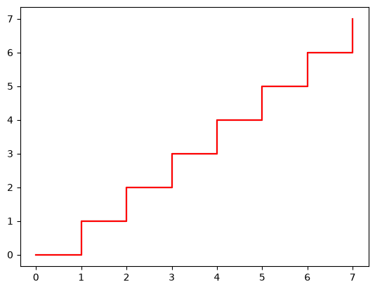
This shows the expected number of events at any time. The model is a step function since it is non-parametric and we have made no assumptions about the count between observed events. The plot also draws pointwise 95% confidence bounds in red (plot_bounds=False hides them, alpha_ci changes their level and ax draws on an existing axes), but with a single item there is no item-to-item variation to measure: the variance estimate is zero and the bounds lie on top of the MCF. One system tells you about that system, not about the population.

The result of this is a Non-Parametric Counting model that can be used just like all other models in surpyval. It is important to note that the fit function takes the values of x as the cumulative time to the event, not the inter-arrival time. If you do have inter-arrival data (which is sorted in the correct order) all you need do is take the cumulative sum of the observations along the length of the array. For example:

from surpyval.recurrent import NonParametricCounting
import numpy as np

interarrival_times = [1, 1, 2, 4, 3, 1, 2, 1]
x = np.cumsum(interarrival_times)

model = NonParametricCounting.fit(x)

With several items, take the cumulative sum within each item, never across the whole array.

We can then use this model to estimate the number of failures at any time. For example, let’s say we wanted to know how many failures we would expect to see after 10 units of time. We can do this by using the mcf method of the model.

from surpyval.recurrent import NonParametricCounting
import numpy as np

interarrival_times = [1, 1, 2, 4, 3, 1, 2, 1]
x = np.cumsum(interarrival_times)

model = NonParametricCounting.fit(x)
model.mcf(10)

np.float64(4.0)

The above two examples use only one item, but we can get the expected number of events based on data from any number of items. Let’s say we had three items observed until the last event. Let’s do some modelling.

from surpyval.recurrent import NonParametricCounting
import numpy as np

x = [1, 2, 3, 4, 5, 6, 7, 1, 4, 6, 9, 2, 7, 8, 9]
i = [1, 1, 1, 1, 1, 1, 1, 2, 2, 2, 2, 3, 3, 3, 3]

model = NonParametricCounting.fit(x, i=i)
model.plot()

<Axes: >

Here we have the expected number of events over time based on the observations of three different items.

These functions work with censoring as well. We need to keep in mind that the only right censored points we can have for an item is the last. This is because it doesn’t make any sense to have a right censored point followed by another event. The same is true for left censored and truncated data. Therefore the “timeline” for a single item must be coherent for the model to work.

Let’s look at how we can use right censoring.

from surpyval.recurrent import NonParametricCounting
import numpy as np

x = [1, 2, 3, 4, 5, 6, 7, 1, 4, 6, 9, 2, 7, 8, 9]
i = [1, 1, 1, 1, 1, 1, 1, 2, 2, 2, 2, 3, 3, 3, 3]
c = [0, 0, 0, 0, 0, 0, 1, 0, 0, 0, 1, 0, 0, 0, 1]

model = NonParametricCounting.fit(x, i=i, c=c)
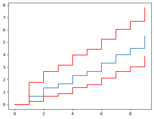
model.plot()

<Axes: >

The fitted model keeps the pieces of the estimate: the distinct observed times x (event and censoring times), the number of items at risk r and the number of events d at each time, the running MCF mcf_hat and its variance var. Item 1 stops being observed at 7, so from time 8 only two items are at risk:

print("x   :", model.x)
print("r   :", model.r)
print("d   :", model.d)
print("MCF :", model.mcf_hat.round(3))

x   : [1. 2. 3. 4. 5. 6. 7. 8. 9.]
r   : [3 3 3 3 3 3 3 2 2]
d   : [2. 2. 1. 2. 1. 2. 1. 1. 0.]
MCF : [0.667 1.333 1.667 2.333 2.667 3.333 3.667 4.167 4.167]

Let’s say this data was for the time, in years, between repairs on home air conditioners of a specific model. We can then use this model to estimate the number of repairs we would need on a newly installed air conditioner. Let’s say we wanted to know how many repairs we would expect to see after 8 years. We can do this by using the mcf method of the model.

model.mcf([8, 10])

array([4.16666667,        nan])

If however, we wanted to know how many repairs were needed after 10 years, we could not do so since the data only goes up to 9 years: the model returns nan rather than guess. To address this we would instead need to use a parametric model.

If you do know that no more repairs happen after the last observed time up to some horizon (or simply want the curve held flat there), say so with set_support(lower, upper). The MCF, and its bounds from mcf_cb, are then 0 from lower to the origin (time 0 here), hold the value at the last observed time up to upper, and are nan outside [lower, upper], for either interp. The bounds must contain the origin and the last observed time; either may be infinite. set_support returns the model, and to_dict saves the bounds with it. The same method on a CauseSpecificMCF bounds every cause’s MCF.

held = NonParametricCounting.fit(x, i=i, c=c).set_support(-5, 12)
held.mcf([-6, -1, 8, 10, 12, 13])

array([       nan, 0.        , 4.16666667, 4.16666667, 4.16666667,
              nan])

Confidence bounds come from mcf_cb. By default they are two-sided 95% bounds, returned as [lower, upper] columns and computed on the log scale so they cannot go negative (bound_type="normal" gives the symmetric estimate \(\pm\) z standard errors instead); bound="lower" or "upper" gives a one-sided bound and alpha_ci sets the level (the default 0.05 gives 95% bounds). The variance behind them is the Lawless-Nadeau robust variance, which allows for items differing in their rates (see Recurrent Event Analysis). mcf and mcf_cb also accept interp="linear" to join the steps with straight lines instead (the estimate and its bounds both rising from 0 at time 0 to the first event):

print("95% bounds at 6.5  :", model.mcf_cb(6.5).round(2))
print("90% upper at 6.5   :", model.mcf_cb(6.5, bound="upper", alpha_ci=0.1).round(2))
print("normal bounds, 6.5 :", model.mcf_cb(6.5, bound_type="normal").round(2))
print("linear MCF at 6.5  :", model.mcf(6.5, interp="linear").round(3))

95% bounds at 6.5  : [1.66 6.7 ]
90% upper at 6.5   : 5.26
normal bounds, 6.5 : [1.01 5.66]
linear MCF at 6.5  : 3.5

The NonParametricCounting model also supports left truncation (delayed entry): an item that was already in service before observation began only joins the at-risk set once its entry time is reached, so events before that entry are estimated over a smaller risk set. Pass the entry time with tl, either as a scalar for every item or as one value per row (the same on every row of an item):

from surpyval.recurrent import NonParametricCounting

x = [2, 3, 5, 3, 4, 6]
i = [1, 1, 1, 2, 2, 2]
c = [0, 0, 1, 0, 0, 1]

model = NonParametricCounting.fit(x, i=i, c=c, tl=1.0)
model.mcf(4)

np.float64(2.0)

Right truncation works the same way at the other end: a finite tr ends an item’s observation there, so the item stays at risk up to tr exactly as it would with an end-of-observation (c=1) row at tr. Here item 1 is watched until 5, so it is still at risk at item 2’s event at 4 even though its own last event was at 3:

x = [2, 3, 3, 4, 6]
i = [1, 1, 2, 2, 2]

model = NonParametricCounting.fit(x, i=i, tr=[5, 5, 8, 8, 8])
print("x :", model.x)
print("r :", model.r)

x : [2. 3. 4. 5. 6. 8.]
r : [2 2 2 2 1 1]

Counts of events (c=2 or c=-1 rows) are not yet supported by the non-parametric risk-set construction; SurPyval raises an error for these rather than return a wrong MCF. For such data use a parametric intensity model.

Trend tests before fitting

Before choosing a parametric model it is worth asking whether the rate of events is changing at all. laplace and mil_hdbk_189c test the null hypothesis of a homogeneous Poisson process (no trend) directly on the event times; no model is fitted. They take the event times x, the item ids i and the observation end T — a scalar, one value per item, or a dict keyed by item. Leave T out for failure-truncated data, and the last event of each item is treated as the end of its window. Data in the fitters’ form, x, i and c, can be passed as they are with c= by keyword: an item’s c = 1 row ends its window (the third positional argument is T, so laplace(x, i, c) raises an error saying so).

from surpyval.recurrent import laplace, mil_hdbk_189c

# inter-arrival times shrinking: failures are speeding up
x = [20, 32, 41, 48, 54, 59, 63, 67, 70, 73, 76, 78, 80, 82, 84]

print(laplace(x, T=85))
print()
print(mil_hdbk_189c(x, T=85, alternative="increasing"))

Laplace Trend Test
==================
Null hypothesis  : no trend (homogeneous Poisson process)
Alternative      : two-sided
Statistic        : 3.04631
p-value          : 0.00231666
Direction        : increasing
Trend            : increasing (p < 0.05)

MIL-HDBK-189C Trend Test
========================
Null hypothesis  : no trend (homogeneous Poisson process)
Alternative      : increasing
Statistic        : 11.4664
DoF              : 30
p-value          : 0.000902298
Direction        : increasing
Trend            : increasing (p < 0.05)

Both tests find strong evidence of an increasing intensity, so an HPP would be a poor model. The alternative argument chooses a two-sided test (the default) or a one-sided test for "increasing" (deterioration) or "decreasing" (reliability growth). The result carries statistic, p_value, direction, trend, n_events and n_systems (and dof for the MIL-HDBK-189C test). direction is only the way the statistic points; trend is the test’s conclusion, "increasing" or "decreasing" only when p_value is below the significance level alpha_ci (default 0.05, set by keyword) and "none" otherwise:

result = laplace([3, 11, 14, 22, 30, 35], T=40)
print(result.direction, "/", result.trend, "- p-value", round(result.p_value, 3))

decreasing / none - p-value 0.86

Here the statistic leans (slightly) towards a decreasing rate, but the p-value is far from small: with six events there is no evidence of any trend, and trend is "none".

Parametric Recurrent Event Models with Surpyval

Just as is the case with single event survival analysis, non-parametric models are not always the best choice. In the case of recurrent events, we can use parametric models to model the number of events at any time. This is done by assuming a form for the intensity of the process. This also has the same limitations as per single event survival analysis. That is, given we use a parametric representation of the intensity we are making assumptions about the shape of the cumulative intensity function. This allows us to extrapolate above the highest observed values but may not be a good fit to the data.

Let’s fit a parametric model.

from surpyval.recurrent import HPP
import numpy as np

x = [1, 2, 3, 4, 5, 6, 7, 1, 4, 6, 9, 2, 7, 8, 9]
i = [1, 1, 1, 1, 1, 1, 1, 2, 2, 2, 2, 3, 3, 3, 3]
c = [0, 0, 0, 0, 0, 0, 1, 0, 0, 0, 1, 0, 0, 0, 1]

model = HPP.fit(x, i=i, c=c)
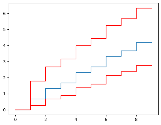
model.plot()

<Axes: >

The plot shows the fitted cumulative intensity (blue) with a shaded 95% confidence band, over the non-parametric MCF of the data (red steps). This model is a good fit to the data, although it is just a straight line. But we can extrapolate above the highest observed value. Let’s say we wanted to know how many events would happen up to “15”, we can do this with the cif method of the model.

model.cif(15)

np.float64(7.2)

This means that we would expect to see 7.2 events up to “15” (in whatever units this model is in): the fitted rate is 12 events in 25 item-time units of observation, 0.48 per unit. Let’s see a different example:

x = [1, 5, 8, 10, 12, 13, 13, 14]
HPP.fit(x).plot()

<Axes: >

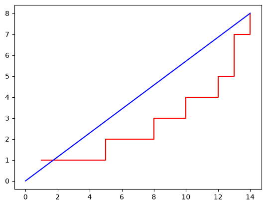
This HPP model, in this case, is not a good fit to the data. This is because the model assumes that the accumulation of events will tend to be a straight line whereas the data appears to be increasing over time. In this case, we have made a poor assumption in using the HPP model. Let’s try another one.

from surpyval.recurrent import Duane
x = [1, 5, 8, 10, 12, 13, 13, 14]

model = Duane.fit(x)
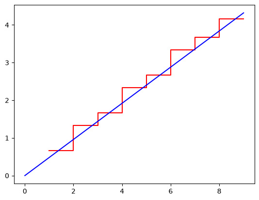
model.plot()

<Axes: >

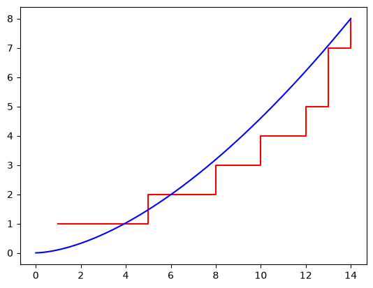
This is clearly a much better fit. The Duane model is a power law, \(\Lambda(t) = b\,t^{\alpha}\); in SurPyval its alpha is the exponent and b the scale:

model

Parametric Recurrence SurPyval Model
==================================
Process             : Duane
Fitted by           : MLE
Parameters          :
     alpha: 1.6436697805495237
         b: 0.10452853873316117

An exponent above one confirms what the plot shows — events are arriving faster as time goes on.

Every fitted intensity model has the same prediction methods: cif (the expected number of events by \(t\)), iif (the instantaneous event rate at \(t\)), mcf (the same as cif for these models) and inv_cif (the time by which a given number of events is expected):

print("expected events by t=20   :", model.cif(20).round(2))
print("event rate at t=20        :", model.iif(20).round(3))
print("time of the 12th event    :", model.inv_cif(12).round(2))

expected events by t=20   : 14.38
event rate at t=20        : 1.182
time of the 12th event    : 17.92

Comparing the intensity models on a fleet

SurPyval has four intensity models: HPP (constant rate), CrowAMSAA and Duane (the power law, in two parameterisations) and CoxLewis (a log-linear intensity). To see how they compare, let’s make data where we know the answer. from_params builds a model from known parameters, and time_terminated_simulation_data simulates items from it, each observed until T (the simulated data ends every item with a c=1 row at T). Here four systems follow a Crow-AMSAA process with \(\alpha = 8\) and \(\beta = 1.6\) and are watched for 50 hours:

from surpyval.recurrent import HPP, CrowAMSAA, Duane, CoxLewis
import numpy as np

true_model = CrowAMSAA.from_params([8.0, 1.6])
data = true_model.time_terminated_simulation_data(50, items=4, random_state=49)
x, i, c = data.x, data.i, data.c
print("events per system:", [int((c[i == k] == 0).sum()) for k in (1, 2, 3, 4)])

events per system: [16, 15, 18, 23]

Now fit each model and compare the information criteria (aic and bic are attributes; lower is better):

fits = {m.name: m.fit(x, i, c) for m in (HPP, CrowAMSAA, Duane, CoxLewis)}
for name, fit in fits.items():
    print(f"{name:28s} AIC {fit.aic:7.2f}   params {fit.params.round(3)}")

Homogeneous Poisson Process  AIC  293.12   params [0.36]
Crow-AMSAA                   AIC  280.63   params [8.432 1.624]
Duane                        AIC  280.63   params [1.624 0.031]
Cox-Lewis                    AIC  281.70   params [-1.888  0.031]

Several lessons are in this small table:

• The HPP is clearly worst: the data has a trend.

• Crow-AMSAA recovers the true parameters well (roughly 8.4 and 1.6) and has the lowest AIC.

• Duane has exactly the same AIC as Crow-AMSAA. It is the same power-law process: its alpha equals Crow-AMSAA’s beta, and its b equals \(\alpha_{CA}^{-\beta_{CA}}\).

• Cox-Lewis is not far behind. Over the observed 50 hours the two shapes are hard to tell apart — but they disagree badly beyond it:

ca, cl = fits["Crow-AMSAA"], fits["Cox-Lewis"]
t = np.array([50.0, 100.0])
print("Crow-AMSAA expected events :", ca.cif(t).round(1))
print("Cox-Lewis  expected events :", cl.cif(t).round(1))
print("true model                 :", true_model.cif(t).round(1))

Crow-AMSAA expected events : [18.  55.5]
Cox-Lewis  expected events : [ 18.  101.8]
true model                 : [18.8 56.9]

Both models agree at 50 hours, where there is data, and differ by a large margin at 100 hours. Extrapolation is only as good as the assumed shape, so check any long-range forecast against more than one plausible model.

Delayed entry and right truncation

Suppose monitoring of the same fleet only started some time after the systems entered service: two were watched from new, two from 20 hours and two from 30 hours, so failures before those times were never recorded. We simulate six systems from the true model and delete what monitoring would have missed. The entry time goes in tl, one value per row:

full = true_model.time_terminated_simulation_data(50, items=6, random_state=48)
entry = {1: 0.0, 2: 0.0, 3: 20.0, 4: 20.0, 5: 30.0, 6: 30.0}
seen = np.array([t >= entry[k] for t, k in zip(full.x, full.i)])
x_d, i_d, c_d = full.x[seen], full.i[seen], full.c[seen]
tl_d = np.array([entry[k] for k in i_d])
print("failures recorded:", int((c_d == 0).sum()), "of", int((full.c == 0).sum()))

print("fit with tl     :", CrowAMSAA.fit(x_d, i_d, c_d, tl=tl_d).params.round(3))
print("tl ignored      :", CrowAMSAA.fit(x_d, i_d, c_d).params.round(3))
print("all failures    :", CrowAMSAA.fit(full.x, full.i, full.c).params.round(3))

failures recorded: 91 of 115
fit with tl     : [8.229 1.643]
tl ignored      : [15.621  2.337]
all failures    : [8.496 1.666]

With tl the likelihood only integrates each system’s intensity from its entry time, and the estimates are close to those from the complete record (the true values are 8 and 1.6). Ignoring the delayed entry treats the unmonitored early hours as hours without failures, which invents a strong wear-out trend (beta about 2.3). The non-parametric MCF corrects for delayed entry through its risk set in the same way:

t = [10, 25, 50]
print("MCF with tl :", NonParametricCounting.fit(x_d, i_d, c_d, tl=tl_d).mcf(t).round(2))
print("tl ignored  :", NonParametricCounting.fit(x_d, i_d, c_d).mcf(t).round(2))
print("true model  :", true_model.cif(t).round(2))

MCF with tl : [ 1.5  6.5 20.5]
tl ignored  : [ 0.5   2.33 15.17]
true model  : [ 1.43  6.19 18.77]

At the other end of the window, tr closes observation without a censoring row: fitting the events with tr=52 gives exactly the time-truncated fit from the start of this page, which used a c=1 row at 52.

print(CrowAMSAA.fit(events, tr=52.0).params.round(3))

[6.706 1.015]

Interval-counted (grouped) data

Sometimes the exact event times are unknown and only the number of events between inspections is recorded. Give each inspection interval as an [start, end] pair in x with c=2, and the number of events found in n. A count of events since new up to a time can be given as a left-censored row (c=-1). The HPP and NHPP models accept these rows, alone or mixed with exact events (when mixing, write an exact event at \(t\) as the pair [t, t] with c=0, and the end of observation as [T, T] with c=1):

from surpyval.recurrent import CrowAMSAA, HPP

# two systems inspected every 10 hours; n is the number of events found
x = [[0, 10], [10, 20], [20, 30], [30, 40]] * 2
n = [2, 3, 5, 6, 1, 4, 4, 7]
i = [1, 1, 1, 1, 2, 2, 2, 2]
c = [2] * 8

grouped = CrowAMSAA.fit(x, i=i, c=c, n=n)
print("Crow-AMSAA params :", grouped.params.round(3))
print("HPP rate          :", HPP.fit(x, i=i, c=c, n=n).params.round(3))

Crow-AMSAA params : [7.96  1.717]
HPP rate          : [0.4]

The HPP rate is the total count divided by the total observed time (32 events in 80 system-hours). The residual diagnostics shown below need exact event times, so they are not available for grouped data.

Least squares, and models from parameters

The NHPP models (CrowAMSAA, Duane, CoxLewis) are fitted by maximum likelihood by default, with the search started from a least-squares fit (init starts it from values of your own instead). how="MSE" stops at that least-squares fit of the cumulative intensity to the non-parametric MCF. It has no likelihood, so AIC, standard errors and confidence bounds are not available for such a fit (the HPP is fitted by maximum likelihood only):

x, i, c = data.x, data.i, data.c
mse = CrowAMSAA.fit(x, i, c, how="MSE")
print("MSE params:", mse.params.round(3))
print("MLE params:", ca.params.round(3))
try:
    mse.aic
except ValueError as err:
    print(err)

MSE params: [9.041 1.696]
MLE params: [8.432 1.624]
Likelihood inference is only available for models fitted from data by maximum likelihood: a how='MSE' fit minimises squared error on the MCF and has no likelihood; refit with how='MLE'.

Similarly, from_params (on HPP, CrowAMSAA, Duane and CoxLewis) builds a model from known parameters without any data. It predicts and simulates like a fitted model, but has no likelihood or data, so inference, diagnostics and plot are not available. Each model’s summary says how it was obtained (Fitted by : MLE, MSE ... or given parameters):

from surpyval.recurrent import HPP

HPP.from_params([0.5])

Parametric Recurrence SurPyval Model
==================================
Process             : Homogeneous Poisson Process
Fitted by           : given parameters (not fitted)
Parameters          :
    lambda: 0.5

Simulating from a fitted model

Any intensity model — fitted, or built with from_params — can simulate new items. There are four methods. The ..._data versions return the simulated events themselves (with x, i, c and n attributes), ready to be refitted; the others return the non-parametric MCF of the simulated items:

• time_terminated_simulation(T, items) / time_terminated_simulation_data(T, items) watch each item until time T;

• count_terminated_simulation(events, items) / count_terminated_simulation_data(events, items) watch each item until it has had events + 1 events (the extra event closes the window). The MCF version keeps only the part of the curve below events, where it is not yet distorted by the items dropping out. A model whose intensity falls away fast enough that its expected number of events over all time, cif(inf), is finite (a CoxLewis with beta < 0) raises a ValueError: an item may never have that many events, so use the time-terminated versions for it.

Pass random_state for a reproducible result. The time-terminated versions also take tol and max_events: a sequence whose gaps shrink below tol (a process heading for an asymptote) or that reaches max_events events before T is stopped at its last event, with a warning. Simulation is a good way to check that a model does what you think, or to see how much data you need to estimate it — here, how precisely one system watched for 50 hours pins down the shape parameter:

betas = []
for seed in range(20):
    sim = true_model.time_terminated_simulation_data(50, items=1, random_state=seed)
    betas.append(CrowAMSAA.fit(sim.x, sim.i, sim.c).params[1])
print("beta estimates from one system: %.2f to %.2f" % (min(betas), max(betas)))

beta estimates from one system: 1.20 to 2.53

A single system gives only a rough idea of the shape; the four-system fleet above did much better.

Expected counts and prediction intervals

The fitted cif is the expected number of events. Its uncertainty, from the uncertainty in the parameters, is given by cif_cb (see the next section). But the actual number of events in a future period is random even if the model is exactly right: for a Poisson process the count in \((t_1, t_2]\) is Poisson distributed with mean \(\Lambda(t_2) - \Lambda(t_1)\). SurPyval has no prediction-interval method, but a plug-in interval takes two lines with scipy. How many failures should one system in our fleet expect in its next 10 hours, from 50 to 60?

from scipy.stats import poisson

expected = float(ca.cif(60) - ca.cif(50))
lower, upper = poisson.ppf([0.05, 0.95], expected)
print(f"expected events in (50, 60]  : {expected:.2f}")
print(f"90% prediction interval      : {lower:.0f} to {upper:.0f}")
print(f"for the fleet of four systems: {poisson.ppf([0.05, 0.95], 4 * expected)}")

expected events in (50, 60]  : 6.20
90% prediction interval      : 2 to 11
for the fleet of four systems: [17. 33.]

Because counts are whole numbers the interval covers at least 90%. This plug-in interval treats the fitted parameters as exact, so with little data it is somewhat too narrow.

Inference and model checking

A fitted parametric recurrence model is more than a point estimate. Every model fit by maximum likelihood exposes the usual likelihood quantities for comparing models — the log-likelihood and the aic / bic information criteria (these are attributes, not methods). Let’s go back to the Duane model of the single system from earlier:

model = Duane.fit([1, 5, 8, 10, 12, 13, 13, 14])
print("log-likelihood:", round(model.log_likelihood, 3))
print("AIC:", model.aic, " BIC:", model.bic)

log-likelihood: -11.634
AIC: 27.268600792751894  BIC: 27.427483876111566

It also carries the uncertainty of the fitted parameters. standard_errors() returns the standard error of each parameter (from the observed information), covariance() the full covariance matrix, and param_cb gives a confidence interval on a named parameter — computed on a transformed scale so the interval respects the parameter’s support (a rate, for instance, cannot go negative):

print("parameters :", model.parameter_names)
print("std errors :", model.standard_errors())
print("alpha 95% CI:", model.param_cb("alpha"))

parameters : ['alpha', 'b']
std errors : [0.58114461 0.16451791]
alpha 95% CI: [0.82197619 3.28677446]

With only eight events the interval on the exponent alpha is wide and includes 1: this single system does not, on its own, prove the rate is increasing.

That parameter uncertainty propagates to the fitted curve. plot() draws a delta-method confidence band around the cumulative intensity function (set plot_bounds=False to hide it, or alpha_ci to change its level), and cif_cb returns the band directly, as [lower, upper] columns. Like every interval in SurPyval, they take the total tail probability alpha_ci (default 0.05, i.e. 95% bounds) rather than a confidence level, and bound="lower" or "upper" gives a one-sided bound:

model.plot()

<Axes: >

model.cif_cb([5, 10, 14])

array([[ 0.37715232,  5.75048823],
       [ 2.08447121, 10.15812185],
       [ 4.0007864 , 15.99692198]])

Having a model is not the same as having a good model. SurPyval provides three complementary checks. First, a trend test on the fitted data — the same Laplace / Military-Handbook tests used to decide whether a time-varying intensity was warranted in the first place (test="mil_hdbk_189c" selects the second, and alternative works as for the standalone functions):

result = model.trend_test()
print(result.direction, "/", result.trend, "- p-value", round(result.p_value, 3))

increasing / none - p-value 0.224

The statistic points to an increasing rate, but with a p-value of about 0.2 the evidence is weak and no trend is concluded at the 5% level — consistent with the wide interval on alpha above.

Second, residuals. Via the time-rescaling theorem, the fitted model turns the event times into what should be a unit-rate Poisson process, so the cumulative-hazard residuals are (under the model) an i.i.d. Exp(1) sample with mean 1:

print(model.residuals().round(3))

[0.105 1.368 1.716 1.413 1.608 0.873 0.    0.917]

(The zero is the second event at 13: two events at the same time are no time apart on any scale.) residuals(kind="pit") transforms them to what should be uniform values, and residuals(kind="martingale") gives one value per item — observed minus expected number of events — which is the easiest way to spot items that fail more (positive) or less (negative) often than the model expects. On the fleet:

print("martingale residuals:", ca.residuals(kind="martingale").round(2))
print("mean of the Exp(1) residuals:", ca.residuals().mean().round(3))

martingale residuals: [-2. -3. -0.  5.]
mean of the Exp(1) residuals: 0.963

The last system had five more failures than the fleet model expects and the second three fewer. For counts of around twenty, whose Poisson standard deviation is between four and five, that is ordinary variation; residuals several times larger would point to a system that is genuinely different. (The mean of the Exp(1) residuals sits a little below one because each system’s final, censored gap — from its last failure to 50 hours — is not part of the residuals; see the caution on the Recurrent Event Analysis page.)

Third, a goodness-of-fit test. cramer_von_mises measures how far the transformed event times fall from uniformity and calibrates the statistic with a parametric bootstrap, so its p-value accounts for the parameters having been estimated. A large p-value means the fitted intensity is consistent with the data. Each bootstrap replicate is a full refit, so keep n_boot modest while exploring (the default is 200):

gof = model.cramer_von_mises(n_boot=100, random_state=2)
print("statistic", round(gof.statistic, 3), " p-value", round(gof.p_value, 3))

statistic 0.053  p-value 0.693

A p-value of about 0.7 gives no reason to doubt the power law for this system. The result object also records n_boot (the replicates actually used; any failed refits are reported in a warning), n_events and n_systems.

The same inference and diagnostic methods are available on the proportional-intensity regression models and the renewal models below.

Renewal Modelling in SurPyval

In contrast to the above, where the cumulative count of events are assumed to have an underlying rate of occurrence, renewal models assume that there is an underlying distribution of the inter-arrival times where each subsequent inter-arrival time is affected by some restoration factor.

All four renewal models — GeneralizedRenewal, GeneralizedOneRenewal, ARA and ARI — take the same x, i, c and n arrays as the intensity models, plus a dist (the lifetime distribution, Weibull by default) and the model’s own options; ARI takes a baseline intensity model in place of the dist. Each item must be observed from new, with exact event times and at most a final right-censored row. They all return a RenewalModel, which has no closed-form cumulative intensity: its mcf and plot work by simulating many items from the fitted model.

Generalised Renewal Process with SurPyval

Generalized Renewal Process modelling is simple with SurPyval:

from surpyval import Weibull
from surpyval.recurrent import GeneralizedRenewal, NonParametricCounting
import numpy as np

x = np.array([1, 2, 3, 4, 4.5, 5, 5.5, 5.7, 6])

model = GeneralizedRenewal.fit(x, dist=Weibull)
model

Generalized Renewal SurPyval Model
==================================
Distribution        : Weibull
Fitted by           : MLE
Kijima Type         : i
Restoration Factor  : 0.15732122999163628
Parameters          : Wald 95% intervals
           estimate      se  lower 95%  upper 95%
    q        0.1573 0.03311     0.1041     0.2376
    alpha     1.261  0.1238      1.041      1.529
    beta      8.939   2.499      5.168      15.46
Repair test: both perfect and minimal repair rejected: q = 0.1573 is
      between perfect and minimal repair (LR tests, q = 0: p =
      0.000108; q = 1: p = 3.59e-05)

The restoration factor q of about 0.16 means each repair removes most, but not all, of the ageing since the previous repair: the item is better-than-old-but-worse-than-new. The fitted lifetime distribution itself is available as model.model (an ordinary SurPyval distribution, with sf, hf and so on), model.q holds the restoration factor and model.kijima_type the Kijima type. As with the intensity models, init (the restoration factor followed by the distribution’s parameters) starts the search from your own values instead of the built-in starts, and GeneralizedRenewal.fit_from_parameters(params, q, kijima=..., dist=...) builds a model from known values for simulation; GeneralizedOneRenewal, ARA and ARI have the same method (ARI’s takes baseline=).

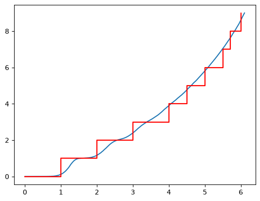
We cannot write down the cumulative intensity function of the model since it does not have a closed form solution. We can however estimate it with a monte carlo simulation of the model. Let’s do that and compare it to a non-parametric description of the MCF:

np_model = model.count_terminated_simulation(len(x), 1000, random_state=1)
ax = np_model.plot()
NonParametricCounting.fit(x).plot(ax=ax)

<Axes: >

We have simulated the model we created up to the number of failures we saw in the data with the count_terminated_simulation method. This method takes two arguments, the first is the number of failures to simulate up to and the second is the number of simulations to run. The more simulations you run the more accurate the model will be. The method returns a NonParametricCounting model that can be used to plot the results. (model.plot() and model.mcf(t) do the same simulation for you, time-terminated at the times of interest; pass items and random_state to control them.)

You can see that the cumulative intensity function of the model is a very good fit to the data. You can also see that it is “wavy.” This is because the underlying distribution is Weibull with a reasonably high shape parameter. This means that the first inter-arrival time is going to be within a relatively narrow period. After the first failure, and the subsequent restoration, the next inter-arrival time is going to be in a larger range since it will be the sum of the first inter-arrival time and the second inter-arrival time. This process continues for each subsequent inter-arrival time. Eventually the waves will become smaller as the mixing of previous inter-arrival times makes the spread of the next inter-arrival time larger and larger. It looks essentially like a smooth line at the higher values.

SurPyval uses the Kijima Type i as the default. Let’s change this to Kijima Type ii and see what happens.

from surpyval import Weibull
from surpyval.recurrent import GeneralizedRenewal, NonParametricCounting
import numpy as np

x = np.array([1, 2, 3, 4, 4.5, 5, 5.5, 5.7, 6])

model_ii = GeneralizedRenewal.fit(x, dist=Weibull, kijima="ii")

np_model = model_ii.count_terminated_simulation(len(x), 1000, random_state=1)
ax = np_model.plot()
NonParametricCounting.fit(x).plot(ax=ax)

<Axes: >

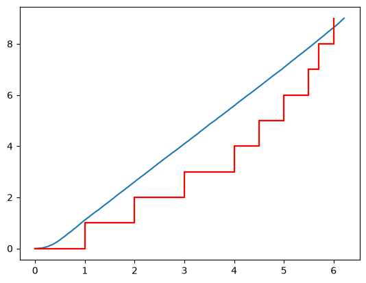
We can see that this model is not as good a fit as the kijima type i model, and the information criteria agree:

print("Kijima i  AIC:", round(model.aic, 2), " q =", round(model.q, 3))
print("Kijima ii AIC:", round(model_ii.aic, 2), " q =", round(model_ii.q, 3))

Kijima i  AIC: -3.66  q = 0.157
Kijima ii AIC: 10.02  q = 0.0

The Kijima-II fit has pushed q to (essentially) zero — perfect repair, an ordinary Weibull renewal process — because Kijima-II’s virtual age, which keeps forgetting old damage, cannot reproduce the steadily shortening gaps between failures the way Kijima-I’s ever-growing age can. This implies that the restoration that is done only repairs damage done since the last event. We could then use this model, via the non-parametric simulations of it, to estimate the number of events up to a given time.

How well do the data determine q?

The restoration factor reads on one scale: q = 0 is a repair as good as new, q = 1 one as bad as old (minimal repair: the process is then the non-homogeneous Poisson process of the distribution’s cumulative hazard, the Crow-AMSAA power law for a Weibull), and q > 1 a repair that leaves the system worse than just before it failed. Only the order and spacing of each system’s failures tell the model about q, so it is often poorly determined, and the printed model gives every parameter’s standard error and Wald 95% interval (model.summary() returns the table). Here eight haul trucks are simulated under minimal repair, so the true q is 1:

rng = np.random.default_rng(8)
rows = []
for k in range(8):
    T = rng.uniform(6000, 12000)
    N = rng.poisson(2e-4 * T**1.35)
    ts = np.sort(T * rng.random(N) ** (1 / 1.35))
    rows += [(h, k, 0) for h in ts] + [(T, k, 1)]
hours, truck, c_trucks = map(np.array, zip(*rows))

trucks = GeneralizedRenewal.fit(hours, truck, c_trucks)
trucks

Generalized Renewal SurPyval Model
==================================
Distribution        : Weibull
Fitted by           : MLE
Kijima Type         : i
Restoration Factor  : 2.6262330531609592
Parameters          : Wald 95% intervals
           estimate     se  lower 95%  upper 95%
    q         2.626  4.469    0.09349      73.78
    alpha     693.6  181.7      415.1       1159
    beta      1.331 0.0986      1.151      1.539
Repair test: consistent with minimal repair; perfect repair rejected
      (LR tests, q = 0: p = 1.72e-09; q = 1: p = 0.528)

The estimate, 2.63, would say every repair makes the truck worse, but its interval runs from 0.09 (almost as good as new) to 74. The question the data can answer is which kinds of repair they rule out, and the last line of the printout answers it: repair_test() refits the model with q held at perfect repair (q = 0, an ordinary Weibull renewal process) and at minimal repair (q = 1, the Crow-AMSAA power law), and tests the fit against each by likelihood ratio:

test = trucks.repair_test()
test

Repair test (likelihood ratio)
==============================
Model               : Generalized Renewal
Estimate            : q = 2.626
Log-likelihood      : -2322.27
Tests               :
        hypothesis value  log-lik LR (df 1)   p-value on edge
    perfect repair q = 0 -2339.73     34.91 1.724e-09     yes
    minimal repair q = 1 -2322.47    0.3983     0.528      no
Conclusion (5% level): consistent with minimal repair; perfect repair
      rejected

print(f"vs perfect: LR = {test.perfect.statistic:.1f}, p = {test.perfect.p_value:.1g}")
print(f"vs minimal: LR = {test.minimal.statistic:.2f}, p = {test.minimal.p_value:.2f}")

vs perfect: LR = 34.9, p = 2e-09
vs minimal: LR = 0.40, p = 0.53

Perfect repair is rejected (p = 2e-9) and minimal repair is not (p = 0.53): the trucks are consistent with minimal repair, and the Crow-AMSAA model, one parameter simpler, describes them as well as the fitted q does. At the level alpha_ci (default 0.05) the conclusion is one of:

• “not determined: the data are consistent with both perfect and minimal repair” – neither is rejected, and the data cannot say what repairs do;

• “consistent with minimal repair; perfect repair rejected”, or the other way round;

• both rejected, and where the estimate lies: “between perfect and minimal repair” (0 < q < 1) or “worse than minimal repair” (q > 1).

Each test has one degree of freedom. Where the value tested is on the edge of the parameter’s range – q = 0 (q cannot be negative), and both rho = 0 and rho = 1 for ARA and ARI – the statistic is a 50:50 mixture of chi-squared(0) and chi-squared(1) when the hypothesis holds, so the p-value is half the chi-squared(1) tail (Self and Liang, 1987). ARA’s rho = 1 is perfect repair; ARI has no repair as good as new, and its rho = 1 (each repair removes all the intensity, the most an ARI repair can) is tested in its place as “maximal repair”. The G1 process has no minimal repair, so it is tested against perfect repair (its q = 0, inside the range) only. The refits are made the first time the model is printed or repair_test() is called, and kept on the model.

A fit can also put the restoration parameter on the edge of its range: a q driven to 0, an ARA or ARI rho to 1 or 0. It then has no standard error, since the likelihood is not regular there, and its interval (param_cb, and the printed table) is the profile-likelihood one: the values the same likelihood-ratio test does not reject, the model refitted at each. It runs from the edge to where twice the drop in the log-likelihood reaches the chi-squared(1) quantile, and a one-sided bound towards the edge is the edge itself. The other parameters’ intervals are then the Wald intervals of the model held on the edge, as the printout notes.

G1 Renewal Process with SurPyval

G1 Modelling can easily be done with SurPyval:

from surpyval import Exponential
from surpyval.recurrent import GeneralizedOneRenewal
import numpy as np
x = np.array([3, 6, 11, 5, 16, 9, 19, 22, 37, 23, 31, 45]).cumsum()

model = GeneralizedOneRenewal.fit(x, dist=Exponential)
model

G1 Renewal SurPyval Model
=========================
Distribution        : Exponential
Fitted by           : MLE
Restoration Factor  : 0.23180803916367387
Parameters          : Wald 95% intervals
                  estimate     se  lower 95%  upper 95%
    q               0.2318 0.1076    0.03797     0.4618
    failure_rate    0.2092 0.1172    0.06973     0.6275
Repair test: perfect repair (a renewal process) rejected: each time
      between failures is 1.232 times the one before (improvement) (LR
      tests, q = 0: p = 0.0191)

This data is from Kaminskiy and Krivtsov’s paper introducing the G1 Renewal Process [1] and shows the inter-arrival times, and not the total time to each event. We therefore need to take the cumulative sum of all the times before passing it to the fit method (the cumulative times are also available as surpyval.datasets.load_g1_kaminskiy_krivtsov()). These are the results the paper reports: \(q \approx 0.232\) and a mean time to the first failure of \(1/0.2092 \approx 4.78\). The inter-arrival times grow over the life of the system, and the positive restoration factor says each repair leaves the system better than new: the expected time to the next failure grows by about 23% with every repair.

Surpyval allows you to use any non-negative lifetime distribution in SurPyval as the underlying distribution. Let’s use the same data with a Weibull G1 Renewal Process.

from surpyval import Weibull
from surpyval.recurrent import GeneralizedOneRenewal, NonParametricCounting
import numpy as np
x = np.array([3, 6, 11, 5, 16, 9, 19, 22, 37, 23, 31, 45]).cumsum()

model = GeneralizedOneRenewal.fit(x, dist=Weibull)
model

G1 Renewal SurPyval Model
=========================
Distribution        : Weibull
Fitted by           : MLE
Restoration Factor  : 0.2163030528695554
Parameters          : Wald 95% intervals
           estimate      se  lower 95%  upper 95%
    q        0.2163 0.03444     0.1506     0.2857
    alpha     5.722   1.038       4.01      8.165
    beta      3.464  0.7952      2.209      5.432
Repair test: perfect repair (a renewal process) rejected: each time
      between failures is 1.216 times the one before (improvement) (LR
      tests, q = 0: p = 6.31e-06)

We can see that the restoration factor is quite similar. What is interesting is that the underlying Weibull distribution has a shape parameter greater than 1. This indicates that the underlying distribution is not exponential. Since the G1 Renewal Process does not have a closed form solution for the cif we can create a non-parametric model from a monte carlo simulation. Let’s do this and compare it to the data MCF.

np_model = model.time_terminated_simulation(250, 1000, random_state=1)
np_model.plot()
NonParametricCounting.fit(x).plot()

<Axes: >

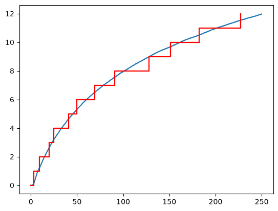
In this code we created a NonParametricCounting model using the G1 Models time_terminated_simulation method. This method takes two arguments, the first is the time to run the simulation to while the second is the number of simulations to run. The more simulations you run the more accurate the model will be. The method returns a NonParametricCounting model that can be used to plot the results. We then also add the raw data to the plot for comparison.

The image above shows that the blue line (the model from the simulation) is in very good agreement to the data. This is a good indication that the underlying distribution is Weibull and that the repair effectiveness has been correctly estimated.

Arithmetic Reduction Models (ARA / ARI) with SurPyval

The ARA (Arithmetic Reduction of Age) and ARI (Arithmetic Reduction of Intensity) models make the memory of a repair explicit through an integer m: how many prior failures an intervention acts on (m=1 by default; numpy.inf for the whole history). ARA reduces a virtual age; ARI reduces the intensity directly. Both are fitted with the same API as the other renewal models, plus the m argument, and both report a repair efficiency rho between 0 (as-bad-as-old) and 1 (as-good-as-new).

To see whether the fit can recover a known answer, we build an ARA model with known parameters using fit_from_parameters — Weibull lifetimes with \(\alpha = 10\) and \(\beta = 3\), repair efficiency \(\rho = 0.5\) and memory \(m = 2\) — and simulate eight systems watched for 40 hours:

from surpyval import Weibull
from surpyval.recurrent import ARA
import numpy as np

ara_true = ARA.fit_from_parameters([10.0, 3.0], 0.5, m=2, dist=Weibull)
sim = ara_true.time_terminated_simulation_data(40, items=8, random_state=3)
x, i, c = sim.x, sim.i, sim.c
print("simulated failures:", int((c == 0).sum()))

model = ARA.fit(x, i, c, dist=Weibull, m=2)
model

simulated failures: 79

ARA Renewal SurPyval Model
==========================
Distribution        : Weibull
Fitted by           : MLE
Memory (m)          : 2
Repair Efficiency   : 0.45311718145382485
Parameters          : Wald 95% intervals
           estimate      se  lower 95%  upper 95%
    rho      0.4531 0.05402     0.3508     0.5595
    alpha     10.63  0.9618      8.899      12.69
    beta      3.096  0.4029      2.399      3.995
Repair test: both perfect and minimal repair rejected: rho = 0.4531 is
      between perfect and minimal repair (LR tests, rho = 1: p =
      2.11e-10; rho = 0: p = 0.000198)

The Repair Efficiency \(\rho\) reported here plays the role of \(1 - q\): a value near 1 is close to as-good-as-new, a value near 0 is as-bad-as-old. The estimates are reasonably close to the values we simulated from (\(\rho = 0.5\), \(\alpha = 10\), \(\beta = 3\)), given about 80 failures.

The memory m is not estimated: it is a choice. A practical way to make it is to fit several values and compare their AIC. m=1 is the Kijima-I model (with \(q = 1 - \rho\)) and m=np.inf the Kijima-II model, so this also compares the two Kijima types:

ara_aic = {}
for m in (1, 2, np.inf):
    fit = ARA.fit(x, i, c, m=m)
    ara_aic[m] = fit.aic
    print(f"m = {m}:  rho = {fit.rho:.3f}   AIC = {fit.aic:.2f}")

m = 1:  rho = 0.676   AIC = 346.09

m = 2:  rho = 0.453   AIC = 343.13

m = inf:  rho = 0.129   AIC = 350.80

The true memory, m=2, has the lowest AIC.

ARI fits the same way but with an intensity (counting process) baseline — CrowAMSAA (the default), Duane or CoxLewis — in place of a lifetime distribution. It is passed as baseline= (dist=, its name before v0.22, still works with a DeprecationWarning until v0.23), and a lifetime distribution there, ARI.fit(x, i, baseline=Weibull), raises an error saying so and naming ARA and GeneralizedRenewal (a Weibull hazard as the baseline intensity is the power law, baseline=CrowAMSAA); the other fitters likewise refuse an intensity model as their lifetime distribution. Here we simulate from an ARI model with a deteriorating power-law baseline (\(\beta = 2.5\)) and fit it back:

from surpyval.recurrent import ARI, CrowAMSAA

ari_true = ARI.fit_from_parameters([10.0, 2.5], 0.6, m=1, baseline=CrowAMSAA)
sim_ari = ari_true.time_terminated_simulation_data(40, items=10, random_state=7)

ari = ARI.fit(sim_ari.x, sim_ari.i, sim_ari.c, baseline=CrowAMSAA, m=1)
ari

ARI Recurrence SurPyval Model
=============================
Baseline Intensity  : Crow-AMSAA
Fitted by           : MLE
Memory (m)          : 1
Repair Efficiency   : 0.5216523509166163
Parameters          : Wald 95% intervals
           estimate     se  lower 95%  upper 95%
    rho      0.5217  0.178     0.2122     0.8153
    alpha     10.42  1.122      8.439      12.87
    beta      2.474 0.2387      2.048      2.989
Repair test: both maximal and minimal repair rejected: rho = 0.5217 is
      between maximal and minimal repair (LR tests, rho = 1: p =
      3.45e-32; rho = 0: p = 0.0368)

The baseline parameters are recovered well (we simulated from \(\alpha = 10\), \(\beta = 2.5\)). The repair efficiency, which we set to 0.6, is estimated less precisely; the standard errors in the next section quantify how precisely.

Checking a renewal model

The renewal models carry the same likelihood inference as the intensity models. The parameter list starts with the repair parameter (q or rho) followed by the lifetime (or baseline) parameters – the order of params and parameter_names too – and the interval on rho is computed on the logit scale so it stays inside (0, 1):

print("parameters :", ari.parameter_names, ari.params.round(3))
print("std errors :", ari.standard_errors().round(3))
print("rho 95% CI :", ari.param_cb("rho").round(3))

parameters : ['rho', 'alpha', 'beta'] [ 0.522 10.422  2.474]
std errors : [0.178 1.122 0.239]
rho 95% CI : [0.212 0.815]

The interval on rho is wide but contains the true 0.6.

The renewal and virtual-age models also carry the same diagnostics as the intensity models. Because they have no marginal cumulative intensity, the residuals come from the conditional intensity — the cumulative hazard accumulated over each interval given the model’s virtual age — but under a well-specified model they are still an i.i.d. Exp(1) sample:

from surpyval import Weibull
from surpyval.recurrent import GeneralizedRenewal
import numpy as np

x = np.array([1, 3, 6, 9, 10, 1.4, 3, 6.7, 8.9, 11, 1, 2.2, 5, 7.5, 9, 12])
i = np.array([1, 1, 1, 1, 1, 2, 2, 2, 2, 2, 3, 3, 3, 3, 3, 3])

model = GeneralizedRenewal.fit(x, i, dist=Weibull, kijima="i")
print("residual mean :", round(model.residuals().mean(), 3))
print("martingale    :", model.residuals(kind="martingale").round(3))
print("trend         :", model.trend_test().trend)

gof = model.cramer_von_mises(n_boot=20, random_state=1)
print("CvM p-value   :", round(gof.p_value, 3))

residual mean : 1.0
martingale    : [ 0.159 -0.739  0.58 ]
trend         : none

CvM p-value   : 0.095

The Cramér–von Mises bootstrap refits the (multi-start) imperfect-repair model once per replicate, so it is noticeably slower than the residual checks; keep n_boot modest while exploring (with 20 replicates the p-value can only be a multiple of 1/21, a coarse answer). Note also that this fit put q at zero — each repair is as good as new — so the model is an ordinary Weibull renewal process. The residuals average exactly one, but that is no evidence of a good fit: every gap here ends in a failure (there are no censoring rows), and for complete data the Weibull maximum-likelihood equations force the cumulative hazards of the gaps to sum to their number. Their pattern (a Q-Q plot against Exp(1), a drift with time) is what carries information. With a p-value of about 0.1 the goodness-of-fit test gives no strong evidence against the model, and the trend test finds no trend (its statistic leans, unconvincingly, towards a decreasing rate).

Predicting with a renewal model

For a renewal model, mcf gives the expected number of events for a new item by simulation (items controls the number of simulated items, default 1000, and random_state makes it reproducible). Because the future depends on the item’s history, a prediction interval for the count also comes from simulation: simulate many new items and read off the spread of their counts. Using the ARA model fitted above:

ara = ARA.fit(sim.x, sim.i, sim.c, m=2)

print("expected failures by t=20, 40:", ara.mcf([20, 40], random_state=1).round(2))

runs = ara.time_terminated_simulation_data(40, items=2000, random_state=2)
counts = np.bincount(runs.i[runs.c == 0].astype(int), minlength=2001)[1:]
print("90% of new systems have between", np.percentile(counts, 5),
      "and", np.percentile(counts, 95), "failures by t=40")

expected failures by t=20, 40: [2.73 9.93]
90% of new systems have between 7.0 and 14.0 failures by t=40

The simulations always start from a new item (virtual age zero), so they answer questions about new units rather than forecasting a specific item’s next failures from its current state.

Gapped (multi-window) observation

Sometimes an item is only observed over a few disjoint windows, with gaps in between during which failures may occur but are not recorded — a vehicle seen only while it is in the depot, for instance. Passing a windows mapping to an intensity model tells SurPyval each item’s observation windows; every event you pass is then an observed failure (c=0), and the windows supply the end-of-window censoring automatically.

from surpyval.recurrent import CrowAMSAA
import numpy as np

# one item, observed on [0, 12] and [20, 40] with an unobserved gap
x = np.array([3, 7, 10, 25, 33, 38])
i = np.array([1, 1, 1, 1, 1, 1])

model = CrowAMSAA.fit(x, i, windows={1: [(0, 12), (20, 40)]})
model.params

array([4.89122538, 0.95836684])

Because Poisson event counts over disjoint windows are independent, each window is fitted as its own observation period; the intensity likelihood and the non-parametric MCF at-risk set both account for the gaps with no extra work. The HPP and NonParametricCounting accept the same windows argument. In the MCF an item simply drops out of the risk set while it is unobserved:

from surpyval.recurrent import NonParametricCounting

x = [3, 7, 10, 25, 33, 5, 14, 22, 35]
i = [1, 1, 1, 1, 1, 2, 2, 2, 2]
windows = {1: [(0, 12), (20, 40)], 2: [(0, 40)]}

mcf = NonParametricCounting.fit(x, i, windows=windows)
print("time    :", mcf.x)
print("at risk :", mcf.r)

time    : [ 3.  5.  7. 10. 12. 14. 22. 25. 33. 35. 40.]
at risk : [2 2 2 2 2 1 2 2 2 2 2]

Item 1 is not at risk at 14, so only one item is counted there. The virtual-age / renewal models reject gapped data, since the virtual age at the start of a later window depends on the unobserved failures during the gap. Every item must appear in windows, windows must not overlap (they may touch), and every event must fall inside one of its item’s windows; windows cannot be combined with tl/tr (or t), covariates or event marks. Because each window is handled as its own observation period, the diagnostics see windows rather than items: residuals(kind="martingale") returns one value per window, and trend_test refuses gapped data, since the trend tests need every system watched from time zero:

gapped = CrowAMSAA.fit([3, 7, 10, 25, 33, 38], [1] * 6,
                       windows={1: [(0, 12), (20, 40)]})
print("martingale residuals, one per window:",
      gapped.residuals(kind="martingale").round(2))

martingale residuals, one per window: [ 0.64 -0.64]

Competing risks: marked recurrent events

When events come in several mutually exclusive types, attach a mark e to each event (use None for censoring rows). As for the univariate competing-risks models, a mark may be any hashable value – a string, an integer, a tuple such as ("pump", 2), or a mix of these – and the causes are listed in a fixed order (a mix of strings and integers by type name, then by text). The non-parametric CauseSpecificMCF gives one mean cumulative function per cause, sharing the at-risk set across causes:

from surpyval.recurrent import CauseSpecificMCF

x = [3, 1, 5, 2, 4, 6]
i = [1, 1, 1, 2, 2, 2]
c = [0, 0, 1, 0, 0, 1]
e = ["A", "B", None, "A", "A", None]   # None marks the censoring rows

model = CauseSpecificMCF.fit(x, i, c, e=e)
ax = model.plot()

Each cause’s curve is an ordinary NonParametricCounting estimate, available as model.models[cause]; mcf and mcf_cb take the cause as their event argument (mcf_cb passes any other keyword, such as alpha_ci or bound, on to that estimate). The data may carry delayed entry (tl), which shrinks the shared risk set, and right truncation (tr), which keeps an item in it up to tr, but, as for the overall MCF, not counts of events. When every event carries a cause, the causes’ MCFs add up to the overall MCF; an event row whose mark is missing counts towards no cause:

print("causes          :", model.event_types)
print("MCF of A at 4.5 :", model.mcf(4.5, "A"))
print("MCF of B at 4.5 :", model.mcf(4.5, "B"))
print("overall at 4.5  :", NonParametricCounting.fit(x, i, c).mcf(4.5))

causes          : ['A', 'B']
MCF of A at 4.5 : 1.5
MCF of B at 4.5 : 0.5
overall at 4.5  : 2.0

For a parametric picture, CauseSpecificNHPP fits one intensity model per cause (CrowAMSAA by default; HPP, Duane and CoxLewis can be passed as dist; how and init are passed on to every cause’s fit). A marked Poisson process decomposes into independent thinned Poisson processes, so each cause is fitted to its own events over the full observation window — other-cause events are ignored, exactly like a censored period. Each item’s window runs from its tl (or zero) to its censoring row, its tr, or failing both its last event. The rows must be exact events or right-censoring rows.

A parametric fit needs more than a handful of events per cause, so let’s build a more realistic data set: five pumps watched for 40 months, suffering seal failures at a roughly constant rate and bearing failures that become more frequent as the pumps wear. We simulate each cause from a Crow-AMSAA process (seal \(\beta = 1\), bearing \(\beta = 2.5\)), mark the events, and add one censoring row per pump at 40:

import numpy as np
from surpyval.recurrent import CrowAMSAA, CauseSpecificMCF, CauseSpecificNHPP

T = 40.0
seal = CrowAMSAA.from_params([6.0, 1.0]).time_terminated_simulation_data(
    T, items=5, random_state=15
)
bearing = CrowAMSAA.from_params([15.0, 2.5]).time_terminated_simulation_data(
    T, items=5, random_state=115
)
s_obs, b_obs = seal.c == 0, bearing.c == 0

x = np.concatenate([seal.x[s_obs], bearing.x[b_obs], np.full(5, T)])
i = np.concatenate([seal.i[s_obs], bearing.i[b_obs], np.arange(1, 6)])
c = np.concatenate([np.zeros(s_obs.sum() + b_obs.sum()), np.ones(5)])
e = ["seal"] * int(s_obs.sum()) + ["bearing"] * int(b_obs.sum()) + [None] * 5

pumps = CauseSpecificNHPP.fit(x, i, c, e=e)
for cause in pumps.event_types:
    print(f"{cause:8s} params (alpha, beta): {pumps.models[cause].params.round(2)}")
print("expected failures per pump by 40, each cause:",
      [round(float(pumps.cif(T, k)), 1) for k in pumps.event_types])
print("expected failures per pump by 40, in total  :",
      round(float(pumps.total_cif(T)), 1))

bearing  params (alpha, beta): [16.89  2.47]
seal     params (alpha, beta): [5.88 1.  ]
expected failures per pump by 40, each cause: [8.4, 6.8]
expected failures per pump by 40, in total  : 15.2

The per-cause shapes tell the maintenance story: seal failures show no trend (beta near 1), bearing failures a strong wear-out trend (beta above 2) — a single model of all failures together would have blurred the two. The cause-specific MCF of the same data is the non-parametric check:

pump_mcf = CauseSpecificMCF.fit(x, i, c, e=e)
ax = pump_mcf.plot()

The dashed steps are each cause’s pointwise confidence bounds (alpha_ci sets the level, plot_bounds=False hides them). They use the same Lawless-Nadeau robust variance as NonParametricCounting.fit (see Recurrent Event Analysis), computed from that cause’s events, so they allow for pumps differing in how often they suffer a cause.

Each pumps.models[cause] is an ordinary fitted recurrence model, so it carries the full cif / iif, inference and diagnostic behaviour shown above; pumps.cif(x, event), pumps.iif(x, event) and pumps.mcf(x, event) are shortcuts, total_cif sums the causes for the overall expected count, and pumps.plot() draws every cause’s fitted cumulative intensity on one axes. For example, a confidence interval on the shape of the bearing failures:

bearing_fit = pumps.models["bearing"]
print("beta 95% CI:", bearing_fit.param_cb("beta").round(2))

beta 95% CI: [1.82 3.34]

The whole interval lies well above 1, so the bearings’ wear-out is not a fluke of this sample.

Both classes also have a fit_from_df method that reads the columns of a pandas DataFrame (x_col, e_col and optionally i_col, c_col, n_col, tl_col, tr_col), as every recurrent fitter does (with e_col for the causes).

Saving and loading a fitted model

Every fitted recurrence model can be serialised to a plain dictionary or a JSON file and rebuilt later. The intensity model is stateless, so only its name and the fitted parameters are stored (for the nonparametric MCF, the step arrays); the reloaded model reproduces every prediction exactly. This works for the parametric intensity fits (CrowAMSAA / Duane / CoxLewis / HPP), the nonparametric MCF, the proportional-intensity regression, the two cause-specific containers, and the renewal / imperfect-repair models (RenewalModel — generalized renewal, G1 renewal, ARA, ARI).

surpyval.from_dict (and surpyval.from_json) restore any SurPyval model without you needing to know which class wrote it:

import numpy as np
import surpyval
from surpyval.recurrent import CrowAMSAA

events = np.sort(np.random.default_rng(0).uniform(0, 1000, 40))
fitted = CrowAMSAA.fit(events)

blob = fitted.to_dict()                    # -> dict
restored = surpyval.from_dict(blob)        # <- dict
t = np.array([100.0, 500.0, 900.0])
print("match:", np.allclose(fitted.cif(t), restored.cif(t)))

match: True

The renewal models store their family, lifetime distribution, repair parameter and memory or Kijima type, and rebuild their simulator on loading, so the same seed gives the same simulated MCF:

restored_ara = surpyval.from_dict(ara.to_dict())
print(restored_ara.mcf([20, 40], random_state=1).round(2))

[2.73 9.93]

Use to_json / from_json for a file directly. The likelihood-inference state (the fitted data and the log-likelihood) is not serialised, so a reloaded model behaves like a from_params one: it predicts and simulates, but confidence bounds, diagnostics and plot need a re-fit. (A reloaded non-parametric MCF keeps its variance, so mcf_cb still works.)

References

[1]

Kaminskiy, M.P. and Krivtsov, V.V., 2010. G1-renewal process as repairable system model. Reliability: Theory & Applications, 1(3) (issue 18). arXiv:1006.3718.