Non-Parametric SurPyval Modelling

This page is the how-to companion to the Non-Parametric Estimation page, which covers the concepts and mathematics behind the Kaplan-Meier, Nelson-Aalen, Fleming-Harrington and Turnbull estimators. Each section below is a worked scenario; where an example relies on an idea (a risk set, a confidence bound, the Turnbull EM) the theory page explains why it works.

To get started, let’s import some useful packages, as such, for the rest of this page we will assume the following imports have occurred:

import surpyval as surv
import numpy as np
from matplotlib import pyplot as plt

Survival modelling with surpyval is very easy. This page will take you through a series of scenarios that can show you how to use the features of surpyval to get you the answers you need. The first example is if you simply have a list of event times and need to estimate the probability of surviving to a given value.

All four estimators share one interface. Each is an object with a fit() method that takes data in the xcnt format described in Types of Data:

• x: the observed values (a 1-D array), or a 2-D array of [left, right] intervals; alternatively pass the two columns as xl and xr;

• c: the censoring flag of each value: 0 observed, 1 right censored, -1 left censored, 2 interval censored (defaults to all observed);

• n: the number of items with each value (defaults to 1 each);

• t: a 2-D array of [left, right] truncation limits, or equivalently tl and tr (scalars apply to every value).

There are four more, optional, arguments: set_lower_limit (see Starting the curve at zero), and, for the Turnbull estimator only, turnbull_estimator, tol and max_iter (see Arbitrarily Truncated and Censored Data). The other estimators ignore those three.

fit() returns a NonParametric model (see its API page for every method), and every model has the same methods (sf, ff, Hf, cb, plot and so on) whichever estimator made it. In each of the examples below, each of the KaplanMeier, NelsonAalen, or FlemingHarrington can be substituted with any of the others. It is the choice of the analyst which should be used (see Choosing between Kaplan-Meier, Nelson-Aalen and Fleming-Harrington). The Turnbull estimator has additional capabilities that can be used when you have right truncated, left censored, or interval censored data.

Complete Data

Using data of the stress of Bofors steel from Weibull’s original paper we can estimate the reliability, that is, the probability that a sample of steel will survive up to a given applied stress. So what does that mean?

We can find when the steel will break. This is particularly useful when we know the application.

For this example, lets say that the maximum tensile stress our design will see during use is 34 units. Lets try and estimate the proportion that will fail during operation.

For this we can use the Nelson-Aalen estimator of the hazard rate, then convert it to the reliability. This is all done with one easy call.

import surpyval as surv
import numpy as np
from matplotlib import pyplot as plt

x = np.array([32, 33, 34, 35, 36, 37, 38, 39, 40, 42])
n = np.array([10, 33, 81, 161, 224, 289, 336, 369, 383, 389])

# Weibull's measurements are cumulative so we need to transform them
n = np.concatenate([[n[0]], np.diff(n)])

bofors_steel_na = surv.NelsonAalen.fit(x, n=n)

plt.figure(figsize=(10, 7));
plt.ylabel('Survival Probability')
plt.xlabel('Stress [1.275kg/mm2]')
plt.ylim([0, 1])
plt.xlim([31, 42])
plt.step(bofors_steel_na.x, bofors_steel_na.R, where='post')
plt.title('Survival Prob vs Stress of Bofors Steel');

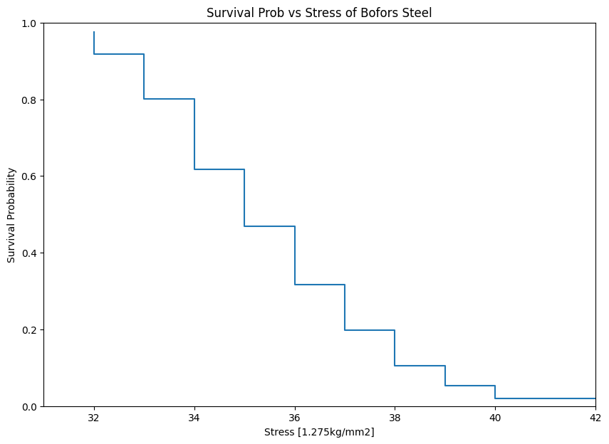
Note the use of n: rather than typing 389 values, each distinct stress is given once with the number of samples that broke there. The step is drawn with where='post' because the estimate drops at each observed value and holds until the next one.

Data held in a pandas DataFrame can be passed with fit_from_df, naming the columns, exactly as for a parametric distribution (x_col, c_col, n_col, xl_col / xr_col and tl_col / tr_col); the estimate is the one fit gives on the same arrays:

import pandas as pd

bofors = pd.DataFrame({'stress': x, 'broke': n})
bofors_df_na = surv.NelsonAalen.fit_from_df(
    bofors, x_col='stress', n_col='broke'
)
print(bofors_df_na.sf([34, 36]).round(4))

[0.8015 0.4689]

So what purpose is this?

With our non-parametric model of the Bofors steel. We can use this model to estimate the reliability in our application. Let’s say that our application uses Bofors steel up to 34. What is our estimate of the number of failures?

print(str(bofors_steel_na.sf(34).round(4).item() * 100) + "%")

80.15%

The above shows that approximately 80% will survive up to a stress of 34. Therefore we will have an approximately 20% chance of our component failing in the design.

It is up to the designer to determine whether this is acceptable.

What if we want to take into account our uncertainty about the reliability. The non-parametric class automatically computes the variance of the estimate using the formula appropriate to the estimator (Greenwood’s formula for Kaplan-Meier, Aalen’s variance for Nelson-Aalen, and the tie-corrected variance for Fleming-Harrington) and uses that to compute the upper and lower confidence intervals. Let’s plot the intervals to see.

plt.figure(figsize=(10, 7))
bofors_steel_na.plot(interp='linear')
plt.xlabel('Stress [1.275kg/mm2]')
plt.ylabel('Survival Probability')
plt.ylim([0, 1])
plt.xlim([32, 42])
plt.title('Surv Prob vs Stress of Bofors Steel')

Text(0.5, 1.0, 'Surv Prob vs Stress of Bofors Steel')

The confidence bounds can also be used to estimate the probability of survival up to some point with some degree of confidence. For example:

lower = bofors_steel_na.cb(34, on='sf', bound='lower', interp='linear', alpha_ci=0.05)
print(str(lower.round(4).item() * 100) + "%")

76.67%

Therefore we can be 95% confident that the reliability at 34 is above 76%. A one-sided bound uses all of alpha_ci on one side, so this lower bound is higher than the lower end of the two-sided 95% interval drawn in the plot. For a Kaplan-Meier model with no right censoring the variance at the final value is undefined with Greenwood’s formula, so the bounds at the last observation are filled with the last finite upper bound and zero for the lower bound. The Nelson-Aalen and Fleming-Harrington variances remain finite at the final value so their bounds are defined all the way to the last observation.

What a fitted model holds

A fitted model stores the estimate in the xrd form described on the theory page: the distinct values x, the number at risk r and the number of failures d at each, and the resulting survival R, failure probability F and cumulative hazard H at each x. Here is a small data set with a tie:

model = surv.KaplanMeier.fit([1, 2, 2, 3, 5, 8])
print(model)
print('x:', model.x)
print('r:', model.r)
print('d:', model.d)
print('R:', model.R.round(4))

Non-Parametric SurPyval Model
=============================
Model            : Kaplan-Meier
Data             : 6 units: 6 events at 5 unique times
x: [1. 2. 3. 5. 8.]
r: [6 5 3 2 1]
d: [1 2 1 1 1]
R: [0.8333 0.5    0.3333 0.1667 0.    ]

Two items fail at 2, so the risk set drops from 5 to 3 across that time and the survival falls by the factor \(1 - 2/5\). The cumulative variance of \(\hat{H}\) behind the confidence bounds is in model.greenwood (the name is historical: for the Nelson-Aalen and Fleming-Harrington estimators it holds their own variance). The raw data the model was fitted with is kept in model.data.

Evaluating the fitted curve

The survival function sf, failure function ff and cumulative hazard Hf can be evaluated anywhere, not just at the observed values. By default they follow the step function (interp='step'): the value at x is the estimate at the largest observed value at or below x, it is 1 before the first observation, and it holds its last value after the last observation.

t = [0, 1, 1.5, 2, 4, 10]
print('sf:', model.sf(t).round(4))
print('ff:', model.ff(t).round(4))
print('linear sf:', model.sf(t, interp='linear').round(4))

sf: [1.     0.8333 0.8333 0.5    0.3333 0.    ]
ff: [0.     0.1667 0.1667 0.5    0.6667 1.    ]
linear sf: [   nan 0.8333 0.6667 0.5    0.25      nan]

interp='linear' (or 'cubic', a shape-preserving interpolant) joins the estimates at the observed values instead; it is nan outside the observed range because there is nothing to interpolate between. Interpolation can make a plot easier to read but is not part of the estimate: the data say nothing about the shape of the curve between observations.

Outside the data, then, what the estimate gives is a convention, and the step function’s (1 before the first value, the last value held however far beyond it) is not always right. When you know the range the variable can take – nothing can have failed before lower, and the curve is to be held flat up to upper – give the model that range with set_support(lower, upper). For every function and every interp, the estimate is then at its start (sf 1; ff, Hf, hf and df 0) from lower to the first observed value, holds its value at the last observed value up to upper, and is nan outside [lower, upper]; the confidence bounds from cb and bootstrap_cb follow the same rule (without a support they are nan outside the data). The bounds must contain the data. lower may be negative (the variable need not be time) and either bound may be infinite. set_support returns the model, so it can follow fit, and to_dict saves the bounds with the model. Without it (model.support is None) nothing changes.

bounded = surv.KaplanMeier.fit([1, 2, 2, 3, 5, 6], c=[0, 0, 0, 0, 0, 1])
bounded = bounded.set_support(0, 10)
t = [-1, 0, 0.5, 4, 8, 10, 11]
print('support:  ', bounded.support)
print('sf:       ', bounded.sf(t).round(4))
print('linear sf:', bounded.sf(t, interp='linear').round(4))
print('cb:\n', bounded.cb(t).round(4))

support:   (0.0, 10.0)
sf:        [   nan 1.     1.     0.3333 0.1667 0.1667    nan]
linear sf: [   nan 1.     1.     0.25   0.1667 0.1667    nan]
cb:
 [[   nan    nan]
 [1.     1.    ]
 [1.     1.    ]
 [0.0461 0.6756]
 [0.0077 0.5168]
 [0.0077 0.5168]
 [   nan    nan]]

Quantiles work on the step function too. qf(p) returns the smallest observed value at which the estimated CDF reaches p, median is qf(0.5) and mean() is the area under the curve (up to the largest observation, by default):

print('10%, 50%, 90% quantiles:', model.qf([0.1, 0.5, 0.9]))
print('median:', model.median)
print('mean:', round(model.mean(), 4))

10%, 50%, 90% quantiles: [1. 2. 8.]
median: 2.0
mean: 3.5

With no censoring the mean is just the sample mean, (1 + 2 + 2 + 3 + 5 + 8)/6 = 3.5. A confidence interval for a quantile comes from quantile_cb(p) (the Brookmeyer-Crowley method: the times at which the pointwise interval for the survival contains \(1 - p\)). It returns one [lower, upper] row per p and takes alpha_ci and bound_type like cb():

print(model.quantile_cb([0.25, 0.5]))

[[ 1.  3.]
 [ 1. nan]]

With six items the data are consistent with a median anywhere from 1 upwards: the upper bound of the survival never falls below 0.5, so the upper end is nan (open). Six items is simply too few to pin a median down.

random(size, random_state=None) draws lifetimes from the fitted estimate: each draw is qf(u) for one uniform u, so each step time is drawn with the probability the estimate puts on it and the draws follow the model’s own sf. If the curve does not reach zero, the probability it leaves beyond its last time is drawn as inf – a lifetime not observed to end within the data, as a parametric model’s never-failing units are:

print(model.random(8, random_state=0))

[2. 5. 8. 8. 2. 1. 2. 2.]

Confidence bounds

cb() returns confidence bounds. By default they are two-sided 95% bounds on the survival function, returned as an array with one [lower, upper] row per requested value:

print(model.cb([1.5, 3, 6]).round(4))

[[0.2731 0.9747]
 [0.0461 0.6756]
 [0.0077 0.5168]]

The options are:

• on: the function to bound, 'sf' (default), 'ff' or 'Hf'. The rows are always [lower, upper] for the function you asked about;

• bound: 'two-sided' (default), 'lower' or 'upper';

• alpha_ci: the significance level, 0.05 by default;

• bound_type: 'exp' (default), the log(-log) interval that always stays within [0, 1], or 'normal', the plain symmetric interval;

• interp: as for sf.

print('on ff:        ', model.cb(3, on='ff').round(4))
print('on Hf:        ', model.cb(3, on='Hf').round(4))
print('90% lower sf: ', model.cb(3, bound='lower', alpha_ci=0.1).round(4))
print("'normal' type:", model.cb(6, bound_type='normal').round(4))
print('at last value:', model.cb(8).round(4))
print('outside data: ', model.cb([0.5, 9]))

on ff:         [0.3244 0.9539]
on Hf:         [0.3922 3.0773]
90% lower sf:  0.116
'normal' type: [-0.1315  0.4649]
at last value: [0.     0.5168]
outside data:  [[nan nan]
 [nan nan]]

The bounds on ff are one minus those on sf (swapped so the lower is still first), and those on Hf are \(-\ln\) of them. The 'normal' interval at 6 runs below zero, which is impossible for a probability and the reason 'exp' is the default. At 8, the last value, the survival estimate is 0 and Greenwood’s variance is undefined, so the lower bound is set to 0 and the upper bound to the last finite one (the upper bound at 5). Outside the range of the data the bounds are nan (unless the model has bounds from set_support, above). The formulas are in the section From a variance to confidence bounds of Non-Parametric Estimation. (cb() also takes dist, but only its default 'z' is accepted; for small samples use bootstrap_cb(), below.)

plot() draws the survival curve with the two-sided bounds as a shaded band, and marks right censored values with ticks. It accepts plot_bounds, show_censors, interp, alpha_ci, bound_type and bound (a one-sided 'lower' or 'upper' bound is drawn as a dashed line), passes anything else (color, label, …) to matplotlib, and can draw on a given ax. The axes are titled with the estimator (“Kaplan-Meier estimate”), the y axis is “Survival probability” and the x axis “Time” unless it already has a label:

fig, ax = plt.subplots(figsize=(8, 5))
model.plot(ax=ax, label='two-sided 95%')
model.plot(ax=ax, bound='lower', alpha_ci=0.1, color='k', label='90% lower bound')
ax.legend();

Starting the curve at zero

A fitted curve starts at the first observed value, so cb() is nan and plot() draws nothing before it. If you know every item was new at some time (usually 0), pass set_lower_limit: it adds that value to the ladder with the full risk set and no failures, so the estimate and its bounds are 1 there. It must be below the smallest value in the data (a ValueError otherwise); it changes nothing else, and it is ignored by the Turnbull estimator.

started = surv.KaplanMeier.fit([1, 2, 2, 3, 5, 8], set_lower_limit=0)
print('x:', started.x, ' r:', started.r, ' d:', started.d)
print('cb at 0.5:', started.cb(0.5))

x: [0. 1. 2. 3. 5. 8.]  r: [6 6 5 3 2 1]  d: [0 1 2 1 1 1]
cb at 0.5: [1. 1.]

Building a model from counts you already have

If your data are already tabulated as times, numbers at risk and numbers of failures (a life table), skip fit() and use from_xrd (available for all but the Turnbull estimator). This is the example ladder from the theory page:

x = [1, 2, 3, 4, 5, 6]
r = [7, 5, 4, 3, 2, 1]
d = [2, 1, 1, 1, 1, 1]

for estimator in [surv.KaplanMeier, surv.FlemingHarrington, surv.NelsonAalen]:
    print(estimator.from_xrd(x, r, d).model, estimator.from_xrd(x, r, d).R.round(4))

Kaplan-Meier [0.7143 0.5714 0.4286 0.2857 0.1429 0.    ]
Fleming-Harrington [0.7338 0.6008 0.4679 0.3353 0.2033 0.0748]
Nelson-Aalen [0.7515 0.6153 0.4792 0.3433 0.2082 0.0766]

The three rows show the ordering \(R_{KM} \leq R_{FH} \leq R_{NA}\) discussed on the theory page. The Kaplan-Meier is one minus the empirical CDF, while the other two never reach zero.

If you only have a survival curve (the values and the survival at each) you can wrap it with surv.NonParametric.fit_from_ecdf(x, R) to get sf, ff, qf and so on (x must be increasing and R non-increasing, within [0, 1]). Without the at-risk and failure counts there is no variance, so such a model cannot produce confidence bounds; draw it with plot(plot_bounds=False).

Plotting positions for probability plots

Probability plotting needs an estimate of \(F\) at each observation. The plotting_positions function returns the x, r, d and F used for that, for any of the rank-based heuristics listed on the theory page or any of the estimators:

from surpyval.univariate.nonparametric import plotting_positions

x = [1, 2, 3, 4, 5, 6, 7, 8]
for heuristic in ['Blom', 'Filliben', 'Mean', 'Nelson-Aalen', 'Kaplan-Meier']:
    _, _, _, F = plotting_positions(x, heuristic=heuristic)
    print(f'{heuristic:>12}:', F.round(3))

        Blom: [0.076 0.197 0.318 0.439 0.561 0.682 0.803 0.924]
    Filliben: [0.083 0.201 0.321 0.44  0.56  0.679 0.799 0.917]
        Mean: [0.111 0.222 0.333 0.444 0.556 0.667 0.778 0.889]
Nelson-Aalen: [0.118 0.235 0.352 0.47  0.587 0.704 0.821 0.934]
Kaplan-Meier: [0.125 0.25  0.375 0.5   0.625 0.75  0.875 1.   ]

Note how the Kaplan-Meier reaches 1 at the largest value (which cannot be plotted on a Weibull axis), while the others stop short of it. plotting_positions also takes c, n and t: right censored data work with every heuristic (the rank based ones use adjusted ranks), left truncation needs one of the estimators, and left or interval censoring or right truncation need heuristic='Turnbull' (with turnbull_estimator to pick the estimator applied to the Turnbull ladder). Anything else raises an error. Here is the rank adjustment at work, with the items at 2 and 5 right censored:

x_pp, _, _, F = plotting_positions([1, 2, 3, 4, 5], c=[0, 1, 0, 0, 1], heuristic='Blom')
print(x_pp, F.round(3))

[1. 2. 3. 4. 5.] [0.119 0.119 0.357 0.595 0.595]

The failure at 1 has rank 1. The censored item at 2 might have failed at any later position, so the failure at 3 gets rank \(1 + (5 + 1 - 1)/(1 + 3) = 2.25\) rather than 3, and the one at 4 gets \(2.25 + (6 - 2.25)/(1 + 2) = 3.5\); Blom’s formula then gives \((2.25 - 0.375)/5.25 = 0.357\) and \((3.5 - 0.375)/5.25 = 0.595\). Censored values are returned too, carrying the previous failure’s value, but only the failures are meant to be plotted. You rarely need to call it yourself: a parametric model’s plot(heuristic=...) and fit(how='MPP', heuristic=...) use it, with 'Nelson-Aalen' as the default (see Parametric SurPyval Modelling).

Saving and restoring a model

A fitted model can be written to a plain dictionary (or a JSON file) and read back, and the restored model has the same curve and bounds. surv.from_dict and surv.from_json work out which kind of model wrote the file:

import json

model_dict = model.to_dict()
restored = surv.from_dict(json.loads(json.dumps(model_dict)))
print(restored.model, restored.sf([1.5, 3]), model.sf([1.5, 3]))

# Keep the data too, so the restored model can bootstrap
with_data = surv.from_dict(json.loads(json.dumps(model.to_dict(with_data=True))))
print(with_data.bootstrap_cb([3], n_boot=50, random_state=0),
      model.bootstrap_cb([3], n_boot=50, random_state=0))

Kaplan-Meier [0.83333333 0.33333333] [0.83333333 0.33333333]
[[0.         0.66666667]] [[0.         0.66666667]]

model.to_json(path) and surv.from_json(path) do the same through a file. By default the raw data are not stored; pass with_data=True to to_dict if the restored model needs to call bootstrap_cb (which refits the data). Without the data a restored model’s plot() draws the curve and bounds but not the censoring ticks. model.to_json(path, with_data=True) keeps the data in a file, to be read back with surv.from_json. The sample size of band() (the number of items fitted) is stored where it differs from the largest risk set, as it does for left truncated data, so the band of a restored model is the original’s (such a dictionary, like one with a support, is schema 2). For Turnbull models the estimator name, tol and max_iter are stored (so a restored model’s bootstrap_cb refits as the original did), but the fitting diagnostics (converged, degenerate and so on) and the bounds, R_upper and R_lower arrays are not.

Right Censored Data

Non-Parametric estimation can handle right censored data. This is possible because at the point of censoring the item is removed from the at risk group without counting a death/failure.

import numpy as np
from surpyval import KaplanMeier as KM

x = np.array([3, 4, 5, 6, 10])
c = np.array([0, 0, 0, 0, 1])
n = np.array([1, 1, 1, 1, 5])

model = KM.fit(x=x, c=c, n=n)
model.R

array([0.88888889, 0.77777778, 0.66666667, 0.55555556, 0.55555556])

model.plot()

<Axes: title={'center': 'Kaplan-Meier estimate'}, xlabel='Time', ylabel='Survival probability'>

In this example, we have included right censored data. This example can be done for the Nelson-Aalen, Fleming-Harrington, and Turnbull estimators as well. The five items still running at 10 never fail in the data, so the curve stops at 0.5556 (drawn with a tick at 10) rather than falling to zero. That has a consequence worth knowing: the estimated CDF never reaches 0.5, so the median (and any quantile above 0.44) is undefined, and surpyval says so rather than guessing:

print('median:', model.median)
print('mean up to 10:', round(model.mean(), 4))

median: nan
mean up to 10: 7.5556

The mean() is the area under the curve up to the largest observation, i.e. the restricted mean over the first 10 units (see Restricted mean survival time).

Choosing between Kaplan-Meier, Nelson-Aalen and Fleming-Harrington

The three estimators agree closely when the risk set is large and failures are not tied, and separate when a large fraction of the risk set fails at once. This data set has many failures tied at the first three times:

x = [1, 2, 3, 4, 5, 6, 7]
c = [0, 0, 0, 1, 0, 0, 1]
n = [6, 4, 2, 2, 1, 1, 2]

fig, ax = plt.subplots(figsize=(8, 5))
for estimator in [surv.KaplanMeier, surv.FlemingHarrington, surv.NelsonAalen]:
    m = estimator.fit(x, c=c, n=n)
    m.plot(ax=ax, plot_bounds=False, label=m.model)
    print(f'{m.model:>18}:', m.sf([1, 2, 6]).round(3))
ax.legend();

      Kaplan-Meier: [0.667 0.444 0.167]
Fleming-Harrington: [0.676 0.46  0.196]
      Nelson-Aalen: [0.717 0.513 0.223]

At time 1, six of eighteen fail. The Kaplan-Meier multiplies by \(1 - 6/18\), the Nelson-Aalen by \(e^{-6/18}\) (noticeably larger) and the Fleming-Harrington splits the tie into six successive failures, landing close to the Kaplan-Meier. After the ties, where one item fails at a time, the Fleming-Harrington drops by the same factor as the Nelson-Aalen. See the section On Surpyval’s recommended estimator of Non-Parametric Estimation for the guidance on which to prefer.

Pointwise bounds, simultaneous bands and the bootstrap

cb() gives pointwise bounds: correct at any one time, but the whole true curve escapes them somewhere more often than 5% of the time. To ask whether a whole curve (say, a fitted Weibull) is consistent with the data, use the simultaneous band from band(). For small samples, or when you distrust the asymptotic formulas, bootstrap_cb() refits the estimator to resampled data. Here is a simulated sample of 60 items with random right censoring:

rng = np.random.default_rng(0)
lifetimes = 10 * rng.weibull(1.5, 60)
censor_times = rng.uniform(0, 20, 60)
x = np.minimum(lifetimes, censor_times)
c = (censor_times < lifetimes).astype(int)

km = surv.KaplanMeier.fit(x, c=c)
t = [5, 10, 15]
print('pointwise:\n', km.cb(t).round(3))
print('Hall-Wellner band:\n', km.band(t).round(3))
print('bootstrap:\n', km.bootstrap_cb(t, n_boot=200, random_state=1).round(3))

pointwise:
 [[0.627 0.862]
 [0.335 0.624]
 [0.11  0.405]]

Hall-Wellner band:
 [[0.567 0.921]
 [0.287 0.691]
 [0.025 0.588]]

bootstrap:
 [[0.646 0.875]
 [0.318 0.628]
 [0.077 0.403]]

The band is wider than the pointwise bounds, as it must be, and the bootstrap interval is close to the pointwise one here, a sign that the asymptotic formula is adequate for this sample. band() takes method='hall-wellner' (default) or method='nair' (the equal-precision band), alpha_ci, and bound_type: the scale the band is applied on, 'arcsine' (the arcsine-square-root of the survival function, the default), 'exp' (its log(-log), as cb()) or 'normal'. Its critical value, that of the limiting Brownian bridge over the range the band covers, is computed numerically rather than simulated, so results are accurate and reproducible. x_range=(t_L, t_U) sets the times a band covers; it is nan outside them. The Hall-Wellner band covers the first to the last event by default. The Nair band’s boundary grows without limit towards the ends of the data, where the estimate rests on a handful of failures or of items at risk, so by default it covers the times where \(a = N\hat{\sigma}^2/(1 + N\hat{\sigma}^2)\) is between 0.1 and 0.9. In simulation it covers 94% to 96% for a nominal 95% so; over the first to the last event it covered 93% on the arcsine scale, 87% to 89% on the log(-log) scale and 83% untransformed, most misses at the first events. bootstrap_cb() takes n_boot (200 resamples), random_state, alpha_ci and a one-sided bound; it always bounds the survival function and, like cb(), is nan outside the range of the data unless the model has a support (set_support).

print('Nair band:\n', km.band(t, method='nair').round(3))
print('Hall-Wellner, normal type:\n', km.band(t, bound_type='normal').round(3))
print('bootstrap 95% lower:', km.bootstrap_cb(t, bound='lower', n_boot=200, random_state=1).round(3))

Nair band:
 [[0.572 0.918]
 [0.27  0.708]
 [0.058 0.506]]
Hall-Wellner, normal type:
 [[ 0.586  0.951]
 [ 0.28   0.696]
 [-0.063  0.551]]

bootstrap 95% lower: [0.656 0.337 0.09 ]

The Nair band follows the shape of the pointwise interval (it is the same formula with a larger critical value), while the Hall-Wellner band’s width follows \(1 + N\hat{\sigma}^2\), so the two distribute their width differently: here the Nair band is a little wider at 10 and narrower at 15. Neither is uniformly better. The 'normal' band, like the 'normal' pointwise interval, can spill below zero (it does at 15); the arcsine and log(-log) bands stay within [0, 1]. With the band we can check a parametric fit against the data:

weibull = surv.Weibull.fit(x, c=c)
band = km.band()          # evaluated at the observed values by default

fig, ax = plt.subplots(figsize=(8, 5))
km.plot(ax=ax, plot_bounds=False, label='Kaplan-Meier')
ax.fill_between(km.x, band[:, 0], band[:, 1], step='post', alpha=0.3,
                label='95% Hall-Wellner band')
grid = np.linspace(0.1, km.x.max(), 200)
ax.plot(grid, weibull.sf(grid), 'k--', label='Weibull fit')
ax.legend();

The Weibull curve stays inside the band, so the data give no reason to reject it.

The hazard rate

A non-parametric cumulative hazard is a step function, so its slope, the hazard rate, has to be approximated. hf() simply takes the change in the cumulative hazard between successive points you ask for, so its values depend on the spacing of your grid (here, steps of 3 units) and are increments rather than rates. smoothed_hf() spreads the jumps of the cumulative hazard with a kernel instead, which is usually what you want; bandwidth (in the units of x) controls the trade-off between smoothness and detail. A hazard needs plenty of data, so here is a larger sample from the same Weibull distribution, whose true hazard is \(0.15 (t/10)^{0.5}\):

rng = np.random.default_rng(0)
lifetimes = 10 * rng.weibull(1.5, 1000)
censor_times = rng.uniform(0, 20, 1000)
big = surv.KaplanMeier.fit(np.minimum(lifetimes, censor_times),
                           c=(censor_times < lifetimes).astype(int))

t = np.array([3, 6, 9, 12])
print('true:        ', (0.15 * (t / 10) ** 0.5).round(3))
print('smoothed_hf: ', big.smoothed_hf(t, bandwidth=3).round(3))
print('hf:          ', big.hf(t).round(3))

true:         [0.082 0.116 0.142 0.164]
smoothed_hf:  [0.072 0.106 0.136 0.134]
hf:           [0.276 0.276 0.363 0.444]

The smoothed estimate follows the true rising hazard, drifting low at 12 where few items remain at risk, while hf() returns increments over 3-unit steps (roughly three times the rate). Note that the first two hf() values are equal: the first point has nothing before it to difference from, so it repeats the second. df() is the drop in the survival over the same step, so it is a grid-dependent probability of failing in each step rather than a density. smoothed_hf() is nan outside the observed range and, if bandwidth is omitted, uses one eighth of that range.

All units survived: success-run testing

A zero-failure test is right censored data in its purest form: every unit is censored at the end of the test. The Kaplan-Meier is then 1 with no variance, which says nothing about the population. success_run answers the useful question instead: after n successes in a row, what reliability can we claim with a given confidence?

from surpyval import success_run

print('10 successes, 95% confidence:', round(success_run(10), 4))
print('59 successes, 95% confidence:', round(success_run(59, confidence=0.95), 4))
print('22 successes, alpha of 0.1:  ', round(success_run(22, alpha=0.1), 4))

10 successes, 95% confidence: 0.7411
59 successes, 95% confidence: 0.9505
22 successes, alpha of 0.1:   0.9006

So 59 consecutive successes demonstrate at least 95% reliability with 95% confidence. Pass either confidence or alpha, not both; the default is 95% confidence.

Left Truncated Data

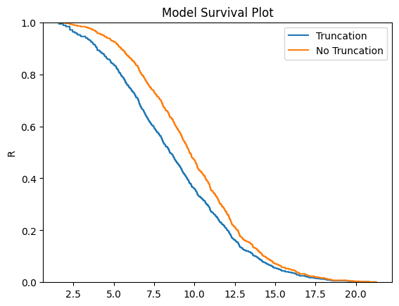
In some instances you will need to account for left truncated data. These data can be passed straight to the same KM, NA, and FH fitters. A common source of left truncation is delayed entry into a study: each subject’s clock starts before they enrol, so anyone who failed before they could enrol is never observed, biasing the sample towards longer survivors. We can simulate such a cohort:

from surpyval import KaplanMeier as KM

np.random.seed(10)
lifetimes = surv.Weibull.random(1_000, 10, 2.5)
entry = np.random.uniform(0, 10, 1_000)

# Only subjects still alive at their entry time are ever enrolled
enrolled = lifetimes > entry
x = lifetimes[enrolled]
tl = entry[enrolled]

model = KM.fit(x=x, tl=tl)
model_no_trunc = KM.fit(x=x)

model.plot(plot_bounds=False)
model_no_trunc.plot(plot_bounds=False)
plt.legend(['Truncation', 'No Truncation'])

<matplotlib.legend.Legend at 0x7bd1ade3a8d0>

The image above shows that if you fail to take into account the left truncation (using the tl keyword) you will overstate the survival probability. This can be used with any of the other non-parametric fitters.

Who is at risk, and when

Truncation works entirely through the risk set: an item is only at risk after it has entered. SurPyval uses the standard \((t_l, x]\) convention, so an item entering at exactly the time of a failure is not at risk for it. Looking at r makes this concrete:

model = KM.fit(x=[2, 3, 3, 4, 5, 6], tl=[0, 0, 1, 1, 2, 2])
print('x:', model.x)
print('r:', model.r)
print('d:', model.d)

x: [2. 3. 4. 5. 6.]
r: [4 5 3 2 1]
d: [1 2 1 1 1]

The two items entering at 2 are not at risk for the failure at 2 (four are), but they are at risk by 3, so the risk set grows from 4 to 5. A value equal to its own entry time would have a zero-length observation window and is rejected with an error. Truncation can also be given as a two-column t array of [left, right] limits, with np.inf for “no right truncation”; this is the same fit:

t = np.array([[0, np.inf], [0, np.inf], [1, np.inf],
              [1, np.inf], [2, np.inf], [2, np.inf]])
print(KM.fit(x=[2, 3, 3, 4, 5, 6], t=t).R.round(4))

[0.75 0.45 0.3  0.15 0.  ]

Two cautions. The estimate is of survival given survival to the earliest entry time; nothing can be said about earlier times. And when few items have entered early the early risk sets are small, so a single early failure moves the curve a long way. Always look at r when you have delayed entry. Right truncation cannot be handled this way (the number at risk is unknown); the Kaplan-Meier, Nelson-Aalen and Fleming-Harrington fitters raise an error and the Turnbull estimator is needed.

Arbitrarily Truncated and Censored Data

In the event you have data that has interval, left, or right censoring with no, left, or right truncation, the previous estimators will not work. Enter the Turnbull estimator. First an interval estimation example:

from surpyval import Turnbull as TB

low = np.array([0, 0, 0, 4, 5, 5, 6, 7, 7, 11, 11, 15, 17, 17,
                17, 18, 19, 18, 22, 24, 24, 25, 26, 27, 32, 33,
                34, 36, 36, 36, 36, 37, 37, 37, 37, 38, 40, 45,
                46, 46, 46, 46, 46, 46, 46, 46])
upp = np.array([7, 8, 5, 11, 12, 11, 10, 16, 14, 15, 18, np.inf,
                np.inf, 25, 25, np.inf, 35, 26, np.inf, np.inf,
                np.inf, 37, 40, 34, np.inf, np.inf, np.inf, 44,
                48, np.inf, np.inf, 44, np.inf, np.inf, np.inf,
                np.inf, np.inf, np.inf, np.inf, np.inf, np.inf,
                np.inf, np.inf, np.inf, np.inf, np.inf])

x = np.array([low, upp]).T
model = TB.fit(x, max_iter=10_000)
model.plot()

<Axes: title={'center': 'Turnbull estimate'}, xlabel='Time', ylabel='Survival probability'>

Each row of x is an interval [left, right] in which the item failed; an upper limit of np.inf means the item was still working at the last inspection (right censored). The censoring flags are worked out from the intervals, so c is not needed. (The same data can be given as TB.fit(xl=low, xr=upp).)

max_iter is raised from its default of 1000 here to leave headroom: with the default Fleming-Harrington option this data takes nearly 900 iterations. The EM stops when no piece’s probability mass changes by more than tol (default 1e-10) in an iteration; loosening tol is the other way to stop sooner, at the cost of accuracy. The Turnbull EM converges slowly when many observations are right censored to infinity, as more than half of these are, and it warns rather than failing silently if it runs out of iterations before reaching tol. If you see that warning, raising max_iter is usually the answer; if it persists, the data may not identify a unique estimate at all. The fitted model records what happened:

print('converged:', model.converged, ' iterations:', model.iters)

converged: True  iterations: 869

And finally, an example with completely arbitrary censoring:

from surpyval import Turnbull as TB

x = [1, 2, [3, 6], 7, 8, 9, [5, 9], [4, 10], [7, 10], 11, 12]
c = [1, 1, 2, 0, 0, 0, 2, 2, 2, -1, 0]
n = [1, 2, 1, 3, 2, 2, 1, 1, 2, 1, 1]

model = TB.fit(x=x, c=c, n=n)
model.plot()

<Axes: title={'center': 'Turnbull estimate'}, xlabel='Time', ylabel='Survival probability'>

With a completely arbitrary set of data we have created a non-parametric estimate of the survival curve that can be used to estimate probabilities. Here x mixes single values and [left, right] pairs, and c says how to read each: right censored at 1 and 2, interval censored in (3, 6], (5, 9], (4, 10] and (7, 10], observed at 7, 8, 9 and 12, and left censored (failed at or before) 11.

Reading a Turnbull model

What is interesting about the Turnbull estimate is that it first finds the data in the ‘xrd’ format. This is done even though we might not have a complete failure occur in an interval. This can be seen by looking at the number of deaths/failures that occur at each value.

print('x:', model.x)
print('d:', model.d.round(3))

x: [ 1.  2.  3.  4.  5.  6.  7.  7.  8.  8.  9.  9. 10. 11. 12. 12.]
d: [0.    0.    0.    0.    0.    1.573 0.    4.711 0.    4.708 0.    4.718
 0.    0.    0.    1.242]

You can see that some values are 0 and that others are fractional: the EM has shared each censored item’s failure out over the times it could have failed at, so d and r are expected counts. The risk set starts at all 17 items, but d adds up to about 16.95: with the default Fleming-Harrington option the curve never reaches zero, so a small share of the two right censored items’ failures is placed beyond the last value (see the theory page). A few things to know when reading them:

• x holds the endpoints of the Turnbull pieces. Exactly observed times appear twice, because the failure mass at such a time sits in the zero-width piece between the two copies.

• d[k] is the expected number of failures in the piece that ends at x[k], i.e. in \((x_{k-1}, x_k]\), and r[k] is the expected number at risk just before that piece, so that R[k] is the estimator applied to r and d up to k, as for the other estimators. So the 1.57 failures at x = 6 are in (5, 6], and the curve drops there. (The first piece starts at model.bounds[0], here \(-\infty\).)

• Where the estimate falls across a piece, the data do not say where in the piece: the drawn step (holding the value until the right end) is a convention. The full set of piece boundaries is model.bounds, and model.R_upper and model.R_lower hold the survival at the start and end of each piece, which is the range any curve through that piece could take:

print('r[0]:', model.r[0].round(3), ' sum of d:', model.d.sum().round(3))
for k in [4, 6]:
    print(f'piece ({model.x[k]:g}, {model.x[k + 1]:g}]: survival between '
          f'{model.R_lower[k]:.3f} and {model.R_upper[k]:.3f}')

r[0]: 17.0  sum of d: 16.953
piece (5, 6]: survival between 0.910 and 1.000
piece (7, 7]: survival between 0.640 and 0.910

The second piece, (7, 7], is the zero-width piece holding the failures observed at exactly 7. The fitted model also records the Turnbull-specific turnbull_estimator, converged, iters, degenerate, npmle and exploitable_mass (described below). Like every other model it carries the cumulative hazard H (\(-\ln R\)), so Hf(), hf(), df() and smoothed_hf() all work as usual.

Choosing the estimator applied to the Turnbull ladder

Because the Turnbull estimate finds the x, r, and d format we can actually elect to use the Nelson-Aalen, Kaplan-Meier or Fleming-Harrington estimate with the Turnbull estimates of x, r, and d, using turnbull_estimator. The default is 'Fleming-Harrington'.

fig, ax = plt.subplots(figsize=(8, 5))
for estimator in ['Kaplan-Meier', 'Fleming-Harrington', 'Nelson-Aalen']:
    m = TB.fit(x=x, c=c, n=n, turnbull_estimator=estimator)
    m.plot(ax=ax, plot_bounds=False, label=estimator)
ax.legend();

The Kaplan-Meier option drops to zero at the last value, as a Kaplan-Meier does, while the Nelson-Aalen and Fleming-Harrington options leave some probability of surviving beyond it, which gives a better approximation for the tail end of the distribution. Only the Kaplan-Meier option is the non-parametric maximum likelihood estimate.

This choice is the usual reason a Turnbull fit does not match a KaplanMeier fit on data both can handle. With the estimator matched, they agree:

x_t = [2, 3, 3, 4, 5, 6]
tl_t = [0, 0, 1, 1, 2, 2]

print('KaplanMeier:        ', KM.fit(x=x_t, tl=tl_t).sf(2))
for estimator in ['Kaplan-Meier', 'Fleming-Harrington', 'Nelson-Aalen']:
    m = TB.fit(x=x_t, tl=tl_t, turnbull_estimator=estimator)
    print(f'Turnbull {estimator:>18}:', m.sf(2).round(4))

KaplanMeier:         0.75
Turnbull       Kaplan-Meier: 0.75
Turnbull Fleming-Harrington: 0.7652
Turnbull       Nelson-Aalen: 0.7788

Compare like with like: pass turnbull_estimator='Kaplan-Meier' when checking a Turnbull fit against KaplanMeier. (A Turnbull fit with the Fleming-Harrington option need not equal FlemingHarrington.fit either, because the Turnbull ladder spreads censored items over later times as fractional failures; see the theory page.)

Confidence bounds for a Turnbull estimate

cb() and plot() work for Turnbull models. For exact and right censored data, with or without left truncation, the variance is computed from the observed counts and matches the Kaplan-Meier’s. With interval or left censoring it treats the expected counts as if they had been observed, which ignores the uncertainty about where the censored failures really were, so the bounds are only approximate. The bootstrap does not have that problem, and is the recommended way to put bounds on such an estimate:

model = TB.fit(x=x, c=c, n=n, turnbull_estimator='Kaplan-Meier')
t = [6, 8, 9]
print('from cb():\n', model.cb(t).round(3))
print('bootstrap:\n', model.bootstrap_cb(t, n_boot=100, random_state=1).round(3))

from cb():
 [[0.629 0.98 ]
 [0.143 0.568]
 [0.006 0.252]]

bootstrap:
 [[0.727 1.   ]
 [0.028 0.716]
 [0.    0.216]]

The bootstrap interval at 8 is much wider than the one from cb(): six of the 17 items were interval or left censored, and the formula-based bound does not know how uncertain their failure times are. Each bootstrap resample refits the Turnbull EM, with the same turnbull_estimator, tol and max_iter as the original fit, so keep n_boot modest for large data sets.

The cb() bounds use the same pieces as the estimate, so they drop where it drops:

print('sf at 5.5:', model.sf(5.5).round(3), ' cb at 5.5:', model.cb(5.5).round(3))
print('sf at 6:  ', model.sf(6).round(3), ' cb at 6:  ', model.cb(6).round(3))

sf at 5.5: 1.0  cb at 5.5: [1. 1.]
sf at 6:   0.907  cb at 6:   [0.629 0.98 ]

The estimate at 5.5 is 1 (the drop in (5, 6] is drawn at 6), and so are both bounds; at 6 all three have dropped.

Truncation with the Turnbull estimator

The Turnbull fitter also accepts truncation (tl/tr, or t). Under truncation the EM iterates with the Kaplan-Meier self-consistency update (the canonical Turnbull M-step), and the requested hazard-form estimator (Fleming-Harrington / Nelson-Aalen) is applied to the converged step function – so on well-sized samples the truncated estimate converges and is well behaved. Here is the mixed-censoring sample again, now with entry times:

tl = [0, 0, 0, 0, 0, 2, 3, 3, 1, 1, 5]

model = TB.fit(x=x, c=c, n=n, tl=tl, max_iter=5_000)
print('converged:', model.converged, ' iterations:', model.iters)
print('degenerate:', model.degenerate, ' npmle:', model.npmle)
print('sf:', model.sf([5, 7, 9, 12]).round(4))

converged: True  iterations: 3320
degenerate: False  npmle: exists
sf: [1.     0.6385 0.0963 0.0155]

This small, truncated, mixed-censoring sample needs about 3,300 iterations; with the default max_iter it would stop early with a warning. Once converged, the diagnostics are clean.

Right truncation arises when items that fail late are never seen, for example when failures are only reported if they happen before a data cut-off. Each item can have its own truncation time:

rng = np.random.default_rng(3)
lifetimes = 10 * rng.weibull(2.0, 300)
cutoff = rng.uniform(5, 20, 300)
seen = lifetimes <= cutoff

model = TB.fit(x=lifetimes[seen], tr=cutoff[seen], turnbull_estimator='Kaplan-Meier')
naive = KM.fit(lifetimes[seen])
t = np.array([4, 8, 12, 16])
print('true:     ', np.exp(-(t / 10) ** 2).round(3))
print('Turnbull: ', model.sf(t).round(3))
print('ignoring truncation:', naive.sf(t).round(3))

true:      [0.852 0.527 0.237 0.077]
Turnbull:  [0.864 0.545 0.219 0.056]
ignoring truncation: [0.813 0.415 0.114 0.016]

Ignoring the truncation badly understates survival, because the long-lived items are exactly the ones that were cut off.

When the data cannot identify the curve

Be aware, though, that the truncated NPMLE is a delicate object: on some data it does not exist (the likelihood only approaches its supremum on the boundary) or is not unique – the data simply do not pin down a unique curve. Which applies is a property of the data, and SurPyval decides it before the EM runs and warns rather than silently returning a meaningless curve:

• npmle is 'exists', 'not unique' (with a warning: some probability is left free, so many curves fit equally well), 'does not exist' (with a warning that the estimate is not identifiable) or 'undetermined' (windows truncated on both sides together with censoring, where the structure alone does not decide);

• degenerate is set, with a warning, if the survival estimate collapses (for example all probability mass escaping below every entry time);

• exploitable_mass is the share of the fitted mass in pieces where mass never lowers the likelihood: some item could have failed there, and every item whose truncation window covers the piece could have too. It is a diagnostic; its size depends on how far the EM got, so the warnings follow npmle;

• converged is False if the EM ran out of iterations (with a warning saying so, unless one of the more specific warnings above was raised instead).

The classic trap is left censoring combined with two or more distinct entry times. Here two of six items are left censored and every item has a different entry time:

import warnings

x_ni = [2, 3, 4, 5, 6, 7]
c_ni = [-1, 0, 0, -1, 0, 0]

with warnings.catch_warnings(record=True) as caught:
    warnings.simplefilter('always')
    bad = TB.fit(x=x_ni, c=c_ni, tl=np.linspace(0.1, 1.0, 6),
                 turnbull_estimator='Kaplan-Meier')
print(caught[0].message.args[0].split(' (')[0] + ' ...')
print('npmle:', bad.npmle, ' converged:', bad.converged)
print('sf:', bad.sf([2, 4, 6]).round(4))

good = TB.fit(x=x_ni, c=c_ni, tl=0.5, turnbull_estimator='Kaplan-Meier')
print('common entry time, sf:', good.sf([2, 4, 6]).round(4))

The Turnbull estimate is not identifiable from this data: the NPMLE does not exist ...
npmle: does not exist  converged: False
sf: [0.005 0.002 0.001]
common entry time, sf: [0.7778 0.3333 0.1667]

The first left censored item could have failed in (0.1, 0.28], before anyone else entered, and nobody who had entered by 0.28 is known to have survived it. Pushing the hazard there towards one raises that item’s likelihood and costs the others nothing (their likelihoods are conditional on their own entry), so the likelihood has no maximum: nearly all of the mass has been pushed there and the survival curve has collapsed. Raising max_iter would not help. With a common entry time the same data fit without complaint. Treat any Turnbull estimate that came with a warning with suspicion. Data that do identify the curve, such as exact failures with right truncation or with staggered entry (unless everyone at risk at some time fails before the next item enters), fit without the warning; the section What the data cannot tell you of Non-Parametric Estimation gives the conditions and where they come from.

Some Issues with the Turnbull Estimate

Caution must be given when using the Turnbull estimate when all values are truncated by some left and/or right value. This is taken up again in the parametric pages. But essentially the Turnbull method cannot make any assumptions about the probability by which the smallest value if left truncated should be adjusted. This is because there is no information available with the non-parametric method below this smallest value. The same is true for the largest value if it is also right truncated, there is no information available about the probability of its observation. Therefore the Turnbull method makes an implicit assumption that the first value, if left truncated has 100% chance of observation, and the highest value, if right truncated also has 100% chance of being observed.

In other words the estimate is conditional on the truncation. When every item has the same right truncation time, the Turnbull estimate is of the distribution given failure before that time, and so it reaches zero there:

x_cut = lifetimes[lifetimes <= 12]
model = TB.fit(x=x_cut, tr=12, turnbull_estimator='Kaplan-Meier')
t = np.array([4, 8, 12])
F12 = 1 - np.exp(-(12 / 10) ** 2)
print('Turnbull:                 ', model.sf(t).round(3))
print('true, given failure by 12:', (1 - (1 - np.exp(-(t / 10) ** 2)) / F12).round(3))

Turnbull:                  [0.834 0.442 0.   ]
true, given failure by 12: [0.806 0.381 0.   ]

The estimate follows the conditional distribution (up to sampling noise), not the unconditional one (whose survival at 12 is about 0.24). The implications of this are detailed in the Parametric section, because the only way to gain an understanding of these situations is by assuming a shape of the distribution. That is, by doing parametric analysis. This is possible since if the distribution within the truncated ends has a shape that matches to a particular distribution you can then extrapolate beyond the observed values. Parametric analysis is therefore incredibly powerful for prediction / extrapolation; see Parametric SurPyval Modelling.

Comparing two groups: the log-rank test

Having estimated a survival curve for each of several groups, the natural next question is whether they differ. The log-rank test is the standard answer: at every event time it compares the observed number of failures in each group with the number expected if all groups shared one survival curve, and combines those differences into a chi-squared statistic with k - 1 degrees of freedom (k groups). A small p-value is evidence the groups differ.

import numpy as np
import surpyval as surv
from surpyval import logrank

np.random.seed(1)
control = surv.Weibull.random(200, 10, 1.2)
treatment = surv.Weibull.random(200, 16, 1.2)   # longer-lived
x = np.concatenate([control, treatment])
group = np.array(['control'] * 200 + ['treatment'] * 200)

result = logrank(x, group)
print(result)

Log-Rank Test
=============
Weighting        : log-rank
Statistic        : 43.3798
DoF              : 1
p-value          : 4.5081e-11

The second argument, Z, holds a group label for each value (any labels will do except NaN or None, which raise an error; with \(k\) distinct labels the test has \(k - 1\) degrees of freedom, counting, as R’s survdiff does, only groups with a positive expected number of failures: a group never at risk at a failure time carries no information). The result’s statistic, dof, p_value and weighting are available as attributes. The test accepts right censored data through c (0 observed, 1 right censored; left or interval censored values raise an error) and counts through n. Here the study is stopped at time 15, so every item still working then is right censored there:

c = (x > 15).astype(int)
x_obs = np.minimum(x, 15)
censored = logrank(x_obs, group, c=c)
print('censored at 15: statistic = %.2f, dof = %d, p = %.3g'
      % (censored.statistic, censored.dof, censored.p_value))

censored at 15: statistic = 34.58, dof = 1, p = 4.09e-09

Censoring removes information, so the statistic is smaller than with the complete data, but the difference is still clear.

weighting chooses the weight given to each event time: 'log-rank' (the default, weight 1), 'gehan' (the number at risk), 'tarone-ware' (its square root) or 'fleming-harrington' with rho and gamma (both 0 by default, which is the plain log-rank). Use them when you expect the difference to be concentrated early or late rather than proportional over time, and pick one before looking at the results:

for weighting in ['log-rank', 'gehan', 'tarone-ware']:
    print(f'{weighting:>12}: p = {logrank(x, group, weighting=weighting).p_value:.3g}')
early = logrank(x, group, weighting='fleming-harrington', rho=1, gamma=0)
print('FH(1, 0), early differences: p = %.3g' % early.p_value)
late = logrank(x, group, weighting='fleming-harrington', rho=0, gamma=1)
print('FH(0, 1), late differences:  p = %.3g' % late.p_value)
print(late.weighting)

    log-rank: p = 4.51e-11
       gehan: p = 2.57e-10
 tarone-ware: p = 6.59e-11
FH(1, 0), early differences: p = 2.57e-10
FH(0, 1), late differences:  p = 2.25e-07
fleming-harrington(rho=0, gamma=1)

These two groups differ by a constant factor in the hazard (the same Weibull shape, a different scale), which is exactly the alternative the plain log-rank is built for, so it gives the smallest \(p\)-value; weights that emphasise only early or only late times lose some power.

Stratified log-rank

When a nuisance factor influences survival — a study site, a batch — comparing groups while ignoring it can be badly misleading if the groups are unevenly distributed across its levels. The stratified log-rank accumulates the observed-minus-expected counts within each stratum before forming the statistic, so groups are only ever compared against others in the same stratum. Pass a strata label per observation.

The example below is confounded on purpose: the baseline hazard differs sharply by site, and the group is unevenly allocated across sites, but there is no true group effect. The pooled test is fooled; the stratified test is not:

np.random.seed(2)
n = 600
site = np.random.randint(0, 2, n)
group = np.where(site == 0, np.random.random(n) < 0.8,
                 np.random.random(n) < 0.2).astype(int)
baseline = np.where(site == 0, 4.0, 20.0)
x = np.random.exponential(baseline)              # no group effect

print('pooled     p = %.4g' % logrank(x, group).p_value)
print(logrank(x, group, strata=site))

pooled     p = 2.181e-14
Stratified Log-Rank Test
========================
Weighting        : log-rank
Strata           : 2
Statistic        : 0.26346
DoF              : 1
p-value          : 0.607753

The stratified result also records the number of strata (its strata attribute). The degrees of freedom are unchanged: stratification changes which items are compared with which, not the number of groups. strata can be combined with c, n and any weighting.

Restricted mean survival time

A hazard ratio (from Cox or the log-rank test) is only interpretable when the proportional-hazards assumption holds. When it does not — survival curves that cross, treatments that help early but not late — the restricted mean survival time (RMST) is an assumption-light alternative. It is simply the area under the survival curve up to a horizon \(\tau\), i.e. the average event-free time over the first \(\tau\) units, and it is always well defined.

Any fitted non-parametric model exposes rmst(tau), returning the point estimate with its standard error and confidence interval:

from surpyval import KaplanMeier

control_model = KaplanMeier.fit(control)
rmst = control_model.rmst(tau=20)
print('RMST(20) = %.2f  (95%% CI %.2f - %.2f)'
      % (rmst['rmst'], rmst['lower'], rmst['upper']))

RMST(20) = 8.55  (95% CI 7.66 - 9.44)

The returned dictionary has keys 'rmst', 'se', 'lower', 'upper' and 'tau'; alpha_ci sets the interval’s level. mean(tau) returns just the point estimate and mean_cb(tau, alpha_ci) just the interval. If tau is omitted it defaults to the largest observed value, where the curve (with no censoring here) has reached zero, so the RMST is then the ordinary mean:

print('90% interval:', control_model.mean_cb(tau=20, alpha_ci=0.1).round(2))
print('mean over all the data:', round(control_model.mean(), 3),
      ' sample mean:', round(control.mean(), 3))

90% interval: [7.8 9.3]
mean over all the data: 9.206  sample mean: 9.206

The interval is the normal one, \(\widehat{\text{RMST}} \pm z\,\widehat{SE}\). A tau beyond the last observation is allowed but holds the curve at its final value out to tau, which is an extrapolation; keep tau within the data.

To compare two groups, surpyval.rmst_diff gives the difference in RMST with a standard error, confidence interval and two-sided p-value. The horizon defaults to the smaller of the two groups’ largest observed times (their common support):

from surpyval import rmst_diff

treatment_model = KaplanMeier.fit(treatment)
diff = rmst_diff(treatment_model, control_model, tau=20)
print('RMST difference = %.2f  (p = %.4g)'
      % (diff['difference'], diff['p_value']))
print({k: round(v, 3) for k, v in diff.items() if k not in ('difference', 'p_value')})

RMST difference = 4.07  (p = 3.466e-10)
{'se': 0.649, 'lower': 2.799, 'upper': 5.342, 'ratio': 1.476, 'rmst_a': 12.62, 'rmst_b': 8.55, 'tau': 20.0}

The treatment group spends about four more time units event-free over the first twenty — a difference on the natural time scale, with no proportional-hazards assumption required. The difference is the first model’s RMST minus the second’s; the result also holds each group’s RMST ('rmst_a', 'rmst_b'), their 'ratio' (rmst_a / rmst_b), the standard error of the difference ('se', the square root of the sum of the two groups’ variances), the interval ('lower', 'upper', at level alpha_ci) and the 'tau' used. The groups can be fitted with any of the non-parametric estimators, and right censoring and delayed entry are handled by those fits.