Regression Modelling with SurPyval
The time until an event — a failure, death, recovery — will almost always depend on external factors. A bearing may last longer in a cool, clean environment than in a hot, dirty one. A patient’s survival may depend on age, dosage, and comorbidities. The question regression modelling answers is: how much do these factors matter, and in what direction?
Regression survival modelling is fundamentally about capturing the relationship between covariates \(Z\) and the survival distribution. Unlike ordinary regression, we must handle censored observations — items that had not yet failed when we stopped watching them — and we want our model to remain valid as a probability distribution (survival functions must start at 1 and decay to 0).
For the rest of this page we assume the following imports:
import surpyval as surv
import numpy as np
from matplotlib import pyplot as plt
Choosing a regression model family
There are three fundamentally different ways a covariate can affect a survival distribution. Each gives rise to a distinct model family:
Proportional Hazards (PH) — the covariate multiplies the rate of dying:
If \(\phi(Z) = 2\), an individual with that covariate value fails at twice the rate at every instant in time. The shape of the hazard curve is unchanged; only its level shifts. This is the most common choice in medical research.
Accelerated Failure Time (AFT) — the covariate stretches or compresses the time axis:
If \(\phi(Z) = 2\), an individual “ages” at twice the normal rate — reaching at age 10 the same cumulative risk that a baseline individual has at age 20. The entire survival curve shifts left or right on the time axis. This is often a more natural framing in engineering and materials science.
Proportional Odds (PO) — the covariate scales the odds of having failed:
The PO formulation is natural when you think about the problem in terms of odds ratios rather than hazard ratios. A key practical difference from PH: the covariate effect attenuates over time. Early in life, hazard ratios and odds ratios behave similarly; at long follow-up times the PO effect fades as everyone converges toward failure regardless of their covariates. When you believe the PH assumption (“constant hazard ratio for all time”) is too strong, PO is often a better default.
Accelerated Life (AL) — the covariate substitutes the distribution’s life parameter:
This is the standard approach in accelerated life testing (ALT) — reliability testing under elevated stress (high temperature, voltage, humidity) to extract failure data quickly, then extrapolating back to use conditions. The stress relationship \(\phi(Z)\) is chosen from domain knowledge: Arrhenius for thermally-activated failure, Eyring for quantum-mechanical processes, Power Law for voltage or mechanical loading.
For PH, AFT, and PO the covariate function is always the log-linear form,
because the exponential guarantees \(\phi > 0\) for any covariate value and any β — no parameter constraints needed. A positive β makes failure faster; negative makes it slower.
SurPyval supports all four families, each available as pre-built instances for every standard distribution and as factory functions for custom combinations:
Family |
Effect of covariates |
Ready-to-use examples |
|---|---|---|
Proportional Hazards (PH) |
Multiplies the hazard rate \(h(x|Z) = h_0(x)\,\phi(Z)\) |
|
Accelerated Failure Time (AFT) |
Scales the time axis \(H(x|Z) = H_0(\phi(Z)\,x)\) |
|
Proportional Odds (PO) |
Scales the survival odds \(O(x|Z) = O_0(x)\,\phi(Z)\) |
|
Accelerated Life (AL) |
Substitutes the life parameter with a physics-motivated function |
|
Semi-Parametric — Cox Proportional Hazards
The Cox PH model is the most widely used survival regression model in any field. Its central insight is that \(\beta\) can be estimated without specifying the shape of the baseline hazard \(h_0(x)\). The baseline cancels out of a partial likelihood, leaving only the relative ordering of event times. This means you can detect and quantify covariate effects even when you have no idea what the baseline distribution looks like.
The price you pay is that the model is semi-parametric: once you have β, the baseline is estimated non-parametrically (a step function with jumps only at observed event times). This means predictions can only be made within the observed time range, and extrapolation is not possible. If you need to predict far beyond your observed data, a parametric PH model is more appropriate.
In this example we use data from Krivtsov et al., testing tires to failure with seven measured characteristics. We want to know which characteristics significantly affect tire life.
from surpyval.datasets import load_tires_data
from surpyval import CoxPH

tires = load_tires_data()
x = tires['Survival']
c = tires['Censoring']
Z = tires[['Tire age', 'Wedge gauge', 'Interbelt gauge', 'EB2B', 'Peel force',
           'Carbon black (%)', 'Wedge gauge×peel force']]
model = CoxPH.fit(x=x, Z=Z, c=c)
model
Semi-Parametric Regression SurPyval Model
=========================================
Type                : Proportional Hazards
Kind                : Cox
Parameterization    : Semi-Parametric
Parameters          :
   beta_0  :  2.109496593744957
   beta_1  :  -9.686078593632985
   beta_2  :  -10.678095367471132
   beta_3  :  -13.675948413338917
   beta_4  :  -34.294485814734955
   beta_5  :  -48.35286747450824
   beta_6  :  20.84037862912318
We can immediately check which coefficients are statistically significant:
print(model.p_values)
[0.13000628 0.03677433 0.02074066 0.0918419  0.01200102 0.14831534
 0.01867559]
Several covariates are not significant. We can re-fit with only the significant ones, which also improves numerical stability:
Z = tires[['Wedge gauge', 'Interbelt gauge', 'Peel force',
           'Wedge gauge×peel force']]
model = CoxPH.fit(x=x, Z=Z, c=c)
print(model.p_values)
model
[0.02207978 0.01368372 0.00956108 0.01030372]
Semi-Parametric Regression SurPyval Model
=========================================
Type                : Proportional Hazards
Kind                : Cox
Parameterization    : Semi-Parametric
Parameters          :
   beta_0  :  -9.313960179920636
   beta_1  :  -7.0692955566811655
   beta_2  :  -27.413473066028942
   beta_3  :  18.105822313416006
All four coefficients are negative, meaning higher gauge and peel force values reduce the hazard rate (improve life) — except the interaction term, which captures a counteracting combined effect.
Survival curves can be evaluated at any covariate value. Here we compare the mean tire against 10% above and below average:
Z_mean = Z.mean().values
plot_x = np.linspace(x.min(), x.max())
for f in [0.9, 1.0, 1.1]:
    plt.step(plot_x, model.sf(plot_x, Z=Z_mean * f), label=f'{f:.0%}')
plt.legend(title='Covariate scale')
plt.xlabel('Survival time')
plt.ylabel('S(x)')
Text(0, 0.5, 'S(x)')
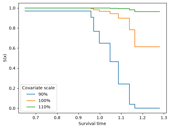
The step-function shape is the signature of the non-parametric baseline — the model makes no smoothness assumptions about \(h_0(x)\).
Parametric Proportional Hazards (PH)
When you are confident about the shape of the baseline distribution — or when you need to extrapolate beyond the observed time range — a fully parametric PH model is preferable. It estimates the same β as the Cox model, but also estimates the baseline distribution parameters, giving a smooth, continuous survival function.
SurPyval provides pre-built parametric PH instances for every standard
distribution: ExponentialPH, NormalPH, WeibullPH, GumbelPH,
LogisticPH, LogNormalPH, and GammaPH. The Weibull is the most
common choice in reliability engineering — its shape parameter lets it capture
increasing, constant, or decreasing hazard rates.
from surpyval import WeibullPH

model = WeibullPH.fit(x=x, Z=Z, c=c)
model
Parametric Regression SurPyval Model
====================================
Kind                : Proportional Hazard
Distribution        : Weibull
Regression Model    : Log Linear [e^(beta'Z)]
Fitted by           : MLE
Distribution        :
     alpha: 0.24255101526650893
      beta: 16.057774400919705
Regression Model    :
    beta_0: -9.165057007955964
    beta_1: -7.998579481971924
    beta_2: -27.50319883629739
    beta_3: 18.385452074179163
Notice the coefficients are very close to the Cox model — this is expected when the Weibull is a reasonable fit to the baseline.
If none of the pre-built distributions suit your data, the PH factory creates
a parametric PH model for any surpyval distribution:
from surpyval import LogNormal
from surpyval import PH

model = PH(LogNormal).fit(x=x, Z=Z, c=c)
model
Parametric Regression SurPyval Model
====================================
Kind                : Proportional Hazard
Distribution        : LogNormal
Regression Model    : Log Linear [e^(beta'Z)]
Fitted by           : MLE
Distribution        :
        mu: 1.9297878812317762e-07
     sigma: 0.15994488851567643
Regression Model    :
    beta_0: -0.33779737213850675
    beta_1: -0.3253514331300051
    beta_2: 1.1385095530825495
    beta_3: -2.281546700228183
The log-normal is a natural choice when the log of the survival time is expected to be normally distributed — common in medical and biological data.
Accelerated Failure Time (AFT)
The AFT model has a different and often more interpretable structure than PH. Rather than saying “this covariate increases your hazard rate by X%”, it says “this covariate makes you age X% faster”. Formally, if the baseline survival time is \(T_0\), then the survival time given covariates is:
A positive \(\beta_j\) means covariate \(z_j\) compresses time (accelerates failure). A negative \(\beta_j\) stretches time (prolongs life). The median survival time simply scales by \(e^{-\beta' Z}\) — a direct and intuitive interpretation.
The relationship to the cumulative hazard is:
An important practical note: for scale-family distributions (Weibull, Log-Normal, Exponential), the Weibull-AFT and Weibull-PH are different parameterisations of the same model family — they will produce equivalent fits with re-parameterised coefficients. For other distributions they are genuinely distinct.
from surpyval import WeibullAFT

model = WeibullAFT.fit(x=x, Z=Z, c=c)
model
Parametric Regression SurPyval Model
====================================
Kind                : Accelerated Failure Time
Distribution        : Weibull
Regression Model    : Log Linear [exp(beta'Z)]
Fitted by           : MLE
Distribution        :
     alpha: 0.2425513511992575
      beta: 16.057759157009166
Regression Model    :
    beta_0: -0.5707541390598181
    beta_1: -0.4981122382953766
    beta_2: -1.7127638829519163
    beta_3: 1.1449550511208184
The AFT factory works with any distribution. Log-Normal AFT is a
particularly common choice — it corresponds to ordinary linear regression on
\(\log T\) with censored observations, and is closely related to the
accelerated failure time model of Buckley & James:
from surpyval import LogNormalAFT

model_ln = LogNormalAFT.fit(x=x, Z=Z, c=c)
model_ln
Parametric Regression SurPyval Model
====================================
Kind                : Accelerated Failure Time
Distribution        : LogNormal
Regression Model    : Log Linear [exp(beta'Z)]
Fitted by           : MLE
Distribution        :
        mu: 5.766405212558384e-16
     sigma: 0.18551241669299862
Regression Model    :
    beta_0: -0.19028013173731836
    beta_1: -0.015546247492115532
    beta_2: 0.20123826580804238
    beta_3: -0.2556419541342986
For distributions not in the pre-built list:
from surpyval import Gamma
from surpyval import AFT

model = AFT(Gamma).fit(x=x, Z=Z, c=c)
model
Parametric Regression SurPyval Model
====================================
Kind                : Accelerated Failure Time
Distribution        : Gamma
Regression Model    : Log Linear [exp(beta'Z)]
Fitted by           : MLE
Distribution        :
     alpha: 88.7934376531835
      beta: 485.1990009358469
Regression Model    :
    beta_0: -0.6121938352911613
    beta_1: -0.6233888476738927
    beta_2: -1.9503487611460653
    beta_3: 1.2516914388183498
We can visualise the “time shift” interpretation by plotting survival curves. The entire curve moves left (shorter life) or right (longer life) on the time axis as the covariates change — a hallmark of the AFT model:
model = WeibullAFT.fit(x=x, Z=Z, c=c)
Z_mean = Z.mean().values
plot_x = np.linspace(x.min(), x.max())
for f in [0.9, 1.0, 1.1]:
    plt.plot(plot_x, model.sf(plot_x, Z=Z_mean * f), label=f'{f:.0%}')
plt.legend(title='Covariate scale')
plt.xlabel('Survival time')
plt.ylabel('S(x)')
Text(0, 0.5, 'S(x)')
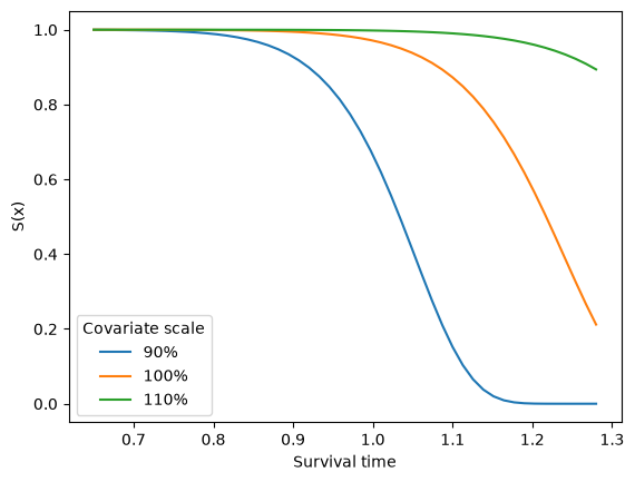
Compare this with the Cox PH survival curves above: the PH curves cross or converge at long times; the AFT curves remain parallel on the log-time scale.
Proportional Odds (PO)
The proportional odds model is less common than PH or AFT but has an important niche: it is the right model when you believe the relative odds of failure are constant across covariate values, rather than the relative hazard rates.
The survival odds at time \(x\) are \(O(x) = S(x) / F(x)\). A PO model assumes these are scaled by \(\phi(Z)\):
Rearranging, the survival function is:
The key difference from PH becomes clear at long follow-up: as \(x \to \infty\), \(S_0(x) \to 0\), and the ratio \(F_0 + \phi S_0 \to 1\), so the covariate effect fades away. Everyone eventually fails, and the PO model respects that by letting the hazard ratio converge to 1 over time. Under PH, the hazard ratio is constant forever — a stronger and often unrealistic assumption for long studies.
PO is the natural companion to the Logistic and Log-Logistic distributions because it corresponds to logistic regression at each time point.
from surpyval import LogisticPO

model = LogisticPO.fit(x=x, Z=Z, c=c)
model
Parametric Regression SurPyval Model
====================================
Kind                : Proportional Odds
Distribution        : Logistic
Regression Model    : Log Linear [exp(beta'Z)]
Fitted by           : MLE
Distribution        :
        mu: -0.5874892941193322
     sigma: 0.06481122986327537
Regression Model    :
    beta_0: 9.754757619554326
    beta_1: 8.864245575260396
    beta_2: 28.02367840471468
    beta_3: -18.71596702847755
The PO factory accepts any distribution:
from surpyval import Weibull
from surpyval import PO

model = PO(Weibull).fit(x=x, Z=Z, c=c)
model
Parametric Regression SurPyval Model
====================================
Kind                : Proportional Odds
Distribution        : Weibull
Regression Model    : Log Linear [exp(beta'Z)]
Fitted by           : MLE
Distribution        :
     alpha: 0.38384753118514925
      beta: 1.932453791706632
Regression Model    :
    beta_0: 3.4795334135351106
    beta_1: 2.2120443577272457
    beta_2: 3.714029108714212
    beta_3: 1.220172836385398
A practical rule of thumb: if the Kaplan-Meier curves for different covariate groups converge at long times (rather than remaining parallel on the log-hazard scale), PO is likely a better fit than PH.
Accelerated Life (AL)
Accelerated life testing (ALT) is a branch of reliability engineering where products are tested under elevated stress conditions — higher temperature, voltage, humidity, or load — to generate failure data faster than would be possible at normal operating conditions. The failures observed at high stress are then extrapolated back to normal conditions using a physical model for how the stress affects the life of the product.
This is fundamentally different from the regression models above. In PH, AFT, and PO, the covariates are measured characteristics of each unit (e.g. tire gauge, patient age). In AL, the covariate is a controlled experimental condition (stress level), and there are typically only two or three distinct levels. The relationship between stress and life is not statistical but physical, and the choice of life model reflects domain knowledge about the failure mechanism.
The AL model substitutes the life parameter \(\theta\) of a distribution with a stress function \(\phi(Z)\):
For example, in a Weibull AL model the scale parameter \(\alpha\) becomes \(\phi(Z)\), while the shape parameter \(\beta\) is estimated globally across all stress levels (the assumption being that the failure mechanism is the same at all stresses, just faster or slower).
Available life models
The choice of life model depends on the physical failure mechanism:
Life model |
Formula \(\phi(Z)\) |
Typical use |
|---|---|---|
|
\(b \cdot e^{a/Z}\) (Arrhenius) |
Thermally-activated (chemical, diffusion, electromigration) |
|
\(Z^{-1} e^{-(c - a/Z)}\) |
Quantum-mechanical processes; more accurate than Arrhenius at extreme temperatures |
|
\(1 / (a \cdot Z^n)\) |
Voltage, electrical field, mechanical fatigue |
|
\(a \cdot Z^n\) |
Same as InversePower but with life increasing with stress |
|
\(a + b \cdot Z\) |
Simple first-order approximation; valid over narrow stress ranges |
|
\(c \cdot e^{a/Z_1} e^{b/Z_2}\) |
Two thermal stresses |
|
\(c \cdot Z_1^m Z_2^n\) |
Two non-thermal stresses |
|
\(c \cdot e^{a/Z_1} Z_2^n\) |
One thermal + one non-thermal |
|
Reciprocal of Eyring |
Inverse Eyring relationship |
|
Reciprocal of Arrhenius |
Inverse Arrhenius relationship |
A note on units: the stress variable \(Z\) for Arrhenius and Eyring should be in Kelvin (absolute temperature), not Celsius.
Using the factory
from surpyval import Weibull
from surpyval import AcceleratedLife, Power, ExponentialLifeModel

# Discrete stress levels — three temperatures in Kelvin
stress = np.array([358.]*20 + [378.]*20 + [398.]*20)  # 85°C, 105°C, 125°C
np.random.seed(42)
# Simulate Arrhenius-like failure times (life halves every ~20°C)
Ea, k = 0.7, 8.617e-5   # activation energy eV, Boltzmann constant eV/K
scale = np.exp(Ea / (k * stress))
x_al = np.random.weibull(2.5, 60) * scale / scale.max() * 5000
c_al = np.ones(60, dtype=int)
c_al[::4] = 1   # every 4th observation right-censored

Z_al = stress.reshape(-1, 1)

# Weibull + Arrhenius (ExponentialLifeModel) — the most common ALT model
model_arr = AcceleratedLife(Weibull, ExponentialLifeModel).fit(x_al, Z=Z_al)
model_arr
Parametric Regression SurPyval Model
====================================
Kind                : Accelerated Life
Distribution        : Weibull
Regression Model    : Exponential
Fitted by           : MLE
Distribution        :
     alpha: 1.0
      beta: 2.351753437317466
Regression Model    :
         a: 7928.647495943155
         b: 1.129832235815103e-06
Notice that the Weibull shape parameter \(\beta\) is estimated globally — it is the same for all stress levels — while the scale parameter \(\alpha\) varies with stress via the Arrhenius relationship. This is the key assumption of ALT: the failure mechanism does not change with stress, only the rate.
# Power law — a common choice for voltage or load acceleration
model_power = AcceleratedLife(Weibull, Power).fit(x_al, Z=Z_al)
model_power
Parametric Regression SurPyval Model
====================================
Kind                : Accelerated Life
Distribution        : Weibull
Regression Model    : Power
Fitted by           : MLE
Distribution        :
     alpha: 1.0
      beta: 2.344738429402598
Regression Model    :
         a: 2.1212918643569032e+57
         n: -21.010910177355345
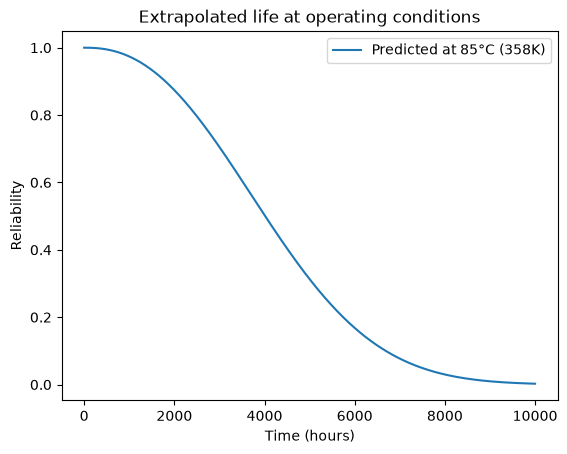
To use the fitted model for extrapolation, pass the operating stress to any of the survival functions:
# Predict life at operating temperature 85°C = 358K
x_pred = np.linspace(0, 10000, 500)
Z_use = np.array([[358.]])   # operating condition

plt.plot(x_pred, model_arr.sf(x_pred, Z=Z_use), label='Predicted at 85°C (358K)')
plt.xlabel('Time (hours)')
plt.ylabel('Reliability')
plt.legend()
plt.title('Extrapolated life at operating conditions')
Text(0.5, 1.0, 'Extrapolated life at operating conditions')
Creating a custom life model
If none of the built-in life models matches your failure physics, you can define
your own by subclassing LifeModel. The two methods you must implement are:
phi(Z, *params)— the stress relationship. Useautograd.numpyso that gradients are available for the optimiser.phi_init(life, Z)— a closed-form or least-squares initialiser for the model parameters.lifeis a vector of estimated life parameters at each unique stress level;Zis the corresponding stress values. Good initialisation is important for convergence.
from surpyval import LifeModel, AcceleratedLife
from surpyval import Weibull
import autograd.numpy as anp

class InverseSquareRoot(LifeModel):
    """Life proportional to 1/sqrt(Z) — a simple custom example."""
    def __init__(self):
        super().__init__(
            name="InverseSquareRoot",
            phi_param_map={"a": 0},
            phi_bounds=((0, None),),
        )

    def phi(self, Z, *params):
        a = params[0]
        return a / anp.sqrt(Z)

    def phi_init(self, life, Z):
        # life ~ a / sqrt(Z) => a ~ life * sqrt(Z)
        a_est = float(anp.mean(life * anp.sqrt(Z.flatten())))
        return [a_est]

model_custom = AcceleratedLife(Weibull, InverseSquareRoot()).fit(x_al, Z=Z_al)
model_custom
Parametric Regression SurPyval Model
====================================
Kind                : Accelerated Life
Distribution        : Weibull
Regression Model    : InverseSquareRoot
Fitted by           : MLE
Distribution        :
     alpha: 1.0
      beta: 1.0541976972774132
Regression Model    :
         a: 38494.634957160306
Model Selection
With several competing models it is useful to compare them on information criteria. AIC penalises log-likelihood by the number of parameters (favouring simpler models); BIC additionally penalises by sample size (favouring even simpler models with larger datasets). Lower is better for both.
For the tires data, we can compare all three statistical regression families using the same Weibull baseline:
from surpyval import WeibullAFT, WeibullPH
from surpyval import PO
from surpyval import Weibull

models = {
    'WeibullPH':  WeibullPH.fit(x=x, Z=Z, c=c),
    'WeibullAFT': WeibullAFT.fit(x=x, Z=Z, c=c),
    'WeibullPO':  PO(Weibull).fit(x=x, Z=Z, c=c),
}

for name, m in models.items():
    print(f'{name:12s}  AIC={m.aic():.2f}  BIC={m.bic():.2f}')
WeibullPH     AIC=-0.04  BIC=2.35
WeibullAFT    AIC=-0.04  BIC=2.35
WeibullPO     AIC=11.81  BIC=14.19
A note of caution: AIC and BIC compare how well a model fits the observed data, not whether the model’s assumptions are correct. A PH model with a lower AIC than a PO model does not mean PH is the “true” model — it means PH uses its parameters more efficiently on this dataset. If the proportional hazards assumption is violated (e.g. survival curves cross), a lower-AIC PH model can still give misleading predictions. Goodness-of-fit diagnostics like Schoenfeld residuals (for PH) or log-log survival plots should accompany any model comparison.